使用scales包自定义ggplot2坐标轴刻度和标签

获取更多R语言知识，请关注公众号：医学和生信笔记

医学和生信笔记，专注R语言在临床医学中的使用，R语言数据分析和可视化。主要分享R语言做医学统计学、meta分析、网络药理学、临床预测模型、机器学习、生物信息学等。

scales包也是Hadley大神开发的R包，主要是作为ggplot2的画图辅助包。

One of the most difficult parts of any graphics package is scaling, converting from data values to perceptual properties. The inverse of scaling, making guides (legends and axes) that can be used to read the graph, is often even harder! The scales packages provides the internal scaling infrastructure used by ggplot2, and gives you tools to override the default breaks, labels, transformations and palettes.

简单来说，在你画图时你可能需要你的坐标轴标签或者其他地方格式是百分比形式，或者小数点后几位，或者特定的标签、单位、颜色色盘的设置等等，这些都可以通过scales包快速实现。

安装

# CRAN:
install.packages("scales")

# Github:
devtools::install_github("r-lib/scales")
1
2
3
4
5

刻度

scales包提供了4个基本函数用于演示一些函数的用法：

• demo_continuous()/demo_log10()：用于连续性数据转换（numerical）
• demo_discrete()：离散型数据
• demo_datetime()：日期时间

这几个设计统一，非常的具有tidy风格，第一个参数指定范围，breaks和labels覆盖默认参数。

下面是一些用法演示，只要你用过ggplot2，你肯定能立刻意会！

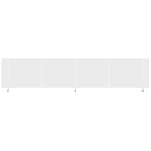
使用breaks_函数控制刻度！

library(scales)

# breaks_width()确定间距
demo_continuous(c(1,10), breaks = breaks_width(2))
## scale_x_continuous(breaks = breaks_width(2))
1
2
3
4
5

如果坐标轴有负数，你不想从0开始，可以使用offset参数：

# 间距是10，从-4开始
demo_continuous(c(0,100),breaks = breaks_width(10, offset = -4))
## scale_x_continuous(breaks = breaks_width(10, offset = -4))
1
2
3

breaks_width函数也可以用于日期时间类型，此时其第一个参数可以是一个带单位的字符串！比如：1 month/3 days/1 week/2 secs/3 hours等等！

one_month <- as.POSIXct(c("2020-05-01", "2020-06-01"))

demo_datetime(one_month)
## scale_x_datetime()
1
2
3
4

demo_datetime(one_month, breaks = breaks_width("5 days"))
## scale_x_datetime(breaks = breaks_width("5 days"))
1
2

demo_datetime(one_month, breaks = breaks_width("1 month"))
## scale_x_datetime(breaks = breaks_width("1 month"))
1
2

# 生成好看的间距，n代表生成几个间距，但是结果可能和你设的不一样
demo_datetime(one_month, breaks = breaks_pretty(n = 4))
## scale_x_datetime(breaks = breaks_pretty(n = 4))
1
2
3

# 使用Wilkinson’s extended breaks algorithm
demo_continuous(c(0,10), breaks = breaks_extended(3))
## scale_x_continuous(breaks = breaks_extended(3))
1
2
3

# log转换使用breaks_logdemo_log10(c(1,1e5), breaks = breaks_log(n=6))## scale_x_log10(breaks = breaks_log(n = 6))
1

demo_discrete(c("a","b","c","d"))## scale_x_discrete()
1

标签

使用label_函数来控制标签的显示，比如几位小数、中间加逗号等。

label_number(accuracy = NULL, scale = 1,              prefix = "", suffix = "",             big.mark = " ", decimal.mark = ".")label_comma(accuracy = NULL, scale = 1,             prefix = "", suffix = "",            big.mark = ",", decimal.mark = ".")            comma(x, accuracy = NULL, scale = 1,       prefix = "", suffix = "",      big.mark = ",", decimal.mark = ".")
1

accuracy：保留几位小数

下面是使用例子：

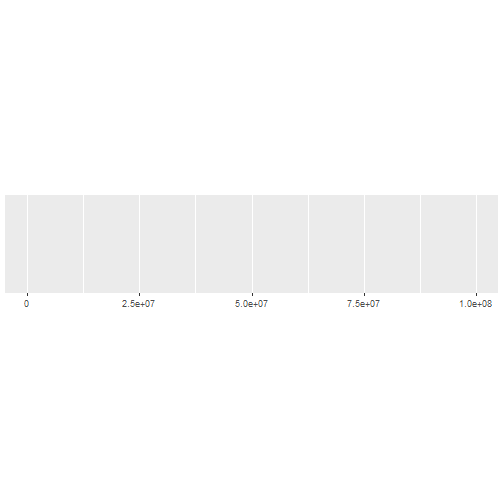
# 不用label_number的情况demo_continuous(c(-1e6, 1e6))## scale_x_continuous()
1

# 使用label_numberdemo_continuous(c(-1e6,1e6), labels = label_number())## scale_x_continuous(labels = label_number())
1

# 每3为数加,demo_continuous(c(-1e6,1e6),labels = label_comma())## scale_x_continuous(labels = label_comma())
1

# 保留1位小数demo_continuous(c(0.20,1.098),labels = label_number(accuracy = 0.1))## scale_x_continuous(labels = label_number(accuracy = 0.1))
1

# 使用scale参数生成更加具有可读性的标签demo_continuous(c(0,1e6),labels = label_number(scale = 1/1e3))## scale_x_continuous(labels = label_number(scale = 1/1000))
1

demo_continuous(c(0, 1e-6), labels = label_number(scale = 1e6,accuracy = 0.001))## scale_x_continuous(labels = label_number(scale = 1e+06, accuracy = 0.001))
1

# 添加后缀demo_continuous(c(32,40),labels = label_number(suffix = "\u00b0C"))## scale_x_continuous(labels = label_number(suffix = "°C"))
1

demo_continuous(c(0,100), labels = label_number(suffix = " kg"))## scale_x_continuous(labels = label_number(suffix = " kg"))
1

# 添加后缀demo_continuous(c(1,10),breaks = breaks_width(2),labels = label_number(prefix = "haha "))## scale_x_continuous(breaks = breaks_width(2), labels = label_number(prefix = "haha "))
1

# 自动添加科学计数法或者10进制格式标签demo_continuous(c(0,1e8), labels = label_number_auto())## scale_x_continuous(labels = label_number_auto())
1

demo_continuous(c(0,1e-3),labels=label_number_auto())## scale_x_continuous(labels = label_number_auto())
1

# 科学计数法demo_continuous(c(0, 1e6), labels = label_scientific())## scale_x_continuous(labels = label_scientific())
1

# 序数demo_continuous(c(1,5), labels = label_ordinal())## scale_x_continuous(labels = label_ordinal())
1

# 支持法语和西班牙语的序数demo_continuous(c(1,5),labels=label_ordinal(rules = ordinal_french()))## scale_x_continuous(labels = label_ordinal(rules = ordinal_french()))
1

# 国际单位制demo_continuous(c(1,1e9),labels = label_number_si())## scale_x_continuous(labels = label_number_si())
1

# 支持换单位demo_continuous(c(1e3,1e6), labels = label_number_si(unit = "g"))## scale_x_continuous(labels = label_number_si(unit = "g"))
1

demo_continuous(c(1,1000), labels = label_number_si(unit = "m"))## scale_x_continuous(labels = label_number_si(unit = "m"))
1

# 百分比样式demo_continuous(c(0,1), labels = label_percent(scale = 100))## scale_x_continuous(labels = label_percent(scale = 100))
1

# 添加美元符号demo_continuous(c(0,1),labels = label_dollar())## scale_x_continuous(labels = label_dollar())
1

demo_continuous(c(0,1),labels = label_dollar(prefix = "USD "))## scale_x_continuous(labels = label_dollar(prefix = "USD "))
1

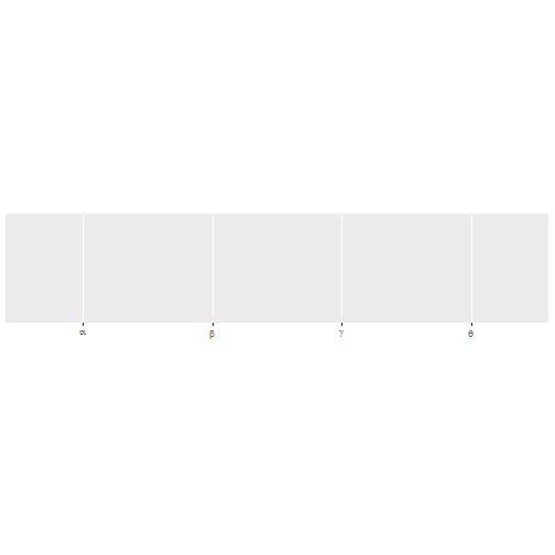
# 数学符号demo_discrete(c("alpha", "beta", "gamma", "theta"),labels = label_parse())## scale_x_discrete(labels = label_parse())
1

# 数字下标demo_continuous(c(1, 5), labels = label_math(alpha[.x]))## scale_x_continuous(labels = label_math(alpha[.x]))
1

# 控制日期时间label_date(format = "%Y-%m-%d", tz = "UTC")label_date_short(format = c("%Y", "%b", "%d", "%H:%M"), sep = "\n")label_time(format = "%H:%M:%S", tz = "UTC")
1

定义一个函数生成一点时间

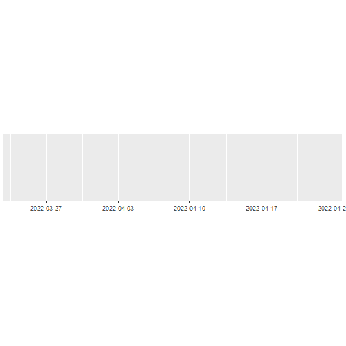
date_range <- function(start, days) {  library(lubridate)  start <- ymd(start)  c(as.POSIXct(start), as.POSIXct(start + days(days)))}library(scales)demo_datetime(date_range("20220325", 30))## scale_x_datetime()## ## 载入程辑包：'lubridate'## The following objects are masked from 'package:base':## ##     date, intersect, setdiff, union
1

demo_datetime(date_range("20220325", 30), labels = label_date())## scale_x_datetime(labels = label_date())
1

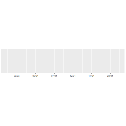
demo_datetime(date_range("20220325", 480),               labels = label_date_short(),               breaks = breaks_width("60 days"))## scale_x_datetime(labels = label_date_short(), breaks = breaks_width("60 days"))
1

对于日期时间，ggplot2提供了两个函数快速定义刻度和标签：date_labels()/date_breaks()。

demo_datetime(date_range("20220325", 30), date_labels = "%d/%m",              date_breaks = "5 days")## scale_x_datetime(date_labels = "%d/%m", date_breaks = "5 days")
1

# 字符创标签label_wrap()x <- c(  "this is a long label",  "this is another long label",  "this a label this is even longer")demo_discrete(x)## scale_x_discrete()
1

# width参数控制每行几个字符demo_discrete(x, labels = label_wrap(width = 5))## scale_x_discrete(labels = label_wrap(width = 5))
1

1个例子

scales包最常用的场景是自定义坐标轴或者图例的标签和刻度。使用break_函数控制如何从一定范围生成刻度，使用label_函数控制如何把刻度转换为标签。

# 加载数据和R包library(ggplot2)library(dplyr)## ## 载入程辑包：'dplyr'## The following objects are masked from 'package:stats':## ##     filter, lag## The following objects are masked from 'package:base':## ##     intersect, setdiff, setequal, unionlibrary(lubridate)glimpse(txhousing)## Rows: 8,602## Columns: 9## $ city       "Abilene", "Abilene", "Abilene", "Abilene", "Abilene", "Abil~## $ year       2000, 2000, 2000, 2000, 2000, 2000, 2000, 2000, 2000, 2000, ~## $ month      1, 2, 3, 4, 5, 6, 7, 8, 9, 10, 11, 12, 1, 2, 3, 4, 5, 6, 7, ~## $ sales      72, 98, 130, 98, 141, 156, 152, 131, 104, 101, 100, 92, 75, ~## $ volume     5380000, 6505000, 9285000, 9730000, 10590000, 13910000, 1263~## $ median     71400, 58700, 58100, 68600, 67300, 66900, 73500, 75000, 6450~## $ listings   701, 746, 784, 785, 794, 780, 742, 765, 771, 764, 721, 658, ~## $ inventory  6.3, 6.6, 6.8, 6.9, 6.8, 6.6, 6.2, 6.4, 6.5, 6.6, 6.2, 5.7, ~## $ date       2000.000, 2000.083, 2000.167, 2000.250, 2000.333, 2000.417, ~
1

# 处理数据df <- txhousing %>%   mutate(date = make_date(year,month,1)) %>%   group_by(city) %>%   filter(min(sales) > 5e2)df## # A tibble: 748 x 9## # Groups:   city [4]##    city    year month sales    volume median listings inventory date      ##                             ##  1 Austin  2000     1  1025 173053635 133700     3084       2   2000-01-01##  2 Austin  2000     2  1277 226038438 134000     2989       2   2000-02-01##  3 Austin  2000     3  1603 298557656 136700     3042       2   2000-03-01##  4 Austin  2000     4  1556 289197960 136900     3192       2.1 2000-04-01##  5 Austin  2000     5  1980 393073774 144700     3617       2.3 2000-05-01##  6 Austin  2000     6  1885 368290072 148800     3799       2.4 2000-06-01##  7 Austin  2000     7  1818 351539312 149300     3944       2.6 2000-07-01##  8 Austin  2000     8  1880 360255090 146300     3948       2.6 2000-08-01##  9 Austin  2000     9  1498 292799874 148700     4058       2.6 2000-09-01## 10 Austin  2000    10  1524 300952544 150100     4100       2.6 2000-10-01## # ... with 738 more rows
1

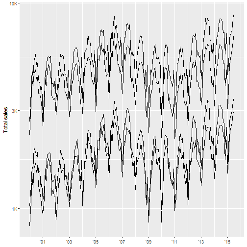
ggplot(df,aes(date, sales, group = city)) +   geom_line(na.rm = TRUE) +   scale_x_date(    NULL,    breaks = scales::breaks_width("2 years"),     labels = scales::label_date("'%y")  ) +   scale_y_log10(    "Total sales",    labels = scales::label_number_si()  )
1

OK，以上就是scales包最常用的功能了，基本上都介绍到了！
但是，你以为这就是它的全部功能了吗？NO NO NO，这只是最常用的功能，它还可以转换颜色/色盘、转换数值等。
还有超多功能大家可以去官网查看学习。

获取更多R语言知识，请关注公众号：医学和生信笔记

医学和生信笔记，专注R语言在临床医学中的使用，R语言数据分析和可视化。主要分享R语言做医学统计学、meta分析、网络药理学、临床预测模型、机器学习、生物信息学等。