-
深度学习实战02-卷积神经网络(CNN)实现服装图像分类
活动地址:CSDN21天学习挑战赛
参考文章:https://mtyjkh.blog.csdn.net/article/details/116992196一、前期准备
1. 设置GPU
如果没有则可不设置,则可以直接使用CPU。
import tensorflow as tf # gpus = tf.config.list_pysical_devices("GPU") # if gpus: # gpu0 = gpus[0] # 如果有多个gpu,仅使用下标为0的那个 # tf.config.experimental.set_memory_growth(gpu0, True) # 设置GPU显存用量按需使用 # tf.config.set_visible_devices([gpu0], "GPU)- 1
- 2
- 3
- 4
- 5
- 6
- 7
2. 导入数据
import tensorflow as tf from tensorflow.keras import datasets, layers, models import matplotlib.pyplot as plt # 下载数据集 (train_images, train_labels), (test_images, test_labels) = datasets.fashion_mnist.load_data()- 1
- 2
- 3
- 4
- 5
- 6
加载数据集会返回四个Numpy数组:
- train_images和train_labels数组是训练集,模型用于学习的数据。
- test_images和test_labels数组是测试集,会被用来对模型进行测试。
图像是28 * 的Numpy数组,像素值介于0-255。标签是整数数组,介于0-9,。这些标签对应于图像所代表的服装类型:
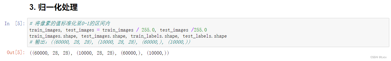
标签 类 标签 类 0 T恤/上衣 1 裤子 2 套头衫 3 连衣裙 4 外套 5 凉鞋 6 衬衫 7 运动鞋 8 包 9 短靴 3. 归一化处理
# 将像素的值标准化至0-1的区间内 train_images, test_images = train_images / 255.0, test_images /255.0 train_images.shape, test_images.shape, train_labels.shape, test_labels.shape # 输出:((60000, 28, 28), (10000, 28, 28), (60000,), (10000,))- 1
- 2
- 3
- 4
4. 调整图片格式
# 调整数据到我们需要的格式 train_images = train_images.reshape((60000, 28, 28, 1)) test_images = test_images.reshape((10000, 28, 28, 1)) train_images.shape, test_images.shape, train_labels.shape, test_labels.shape # 输出:((60000, 28, 28, 1), (10000, 28, 28, 1), (60000,), (10000,))- 1
- 2
- 3
- 4
- 5
- 6

5. 可视化
class_names = ["T-shirt/top", "Trouser", "Pullover", "Dress", "Coat", "Sandal", "Shirt", "Sneaker", "Bag", "Ankle boot"] plt. figure(figsize=(20, 10)) for i in range(20): plt.subplot(5, 10, i +1) plt.xticks([]) plt.yticks([]) plt.grid(False) plt.imshow(train_images[i], cmap=plt.cm.binary) plt.xlabel(class_names[train_labels[i]]) plt.show()- 1
- 2
- 3
- 4
- 5
- 6
- 7
- 8
- 9
- 10
- 11

二、构建CNN网络
卷积神经网络(CNN)的输入是张量(Tensor)形式的(image_height, image_width, color_channels),包含了图像高度、宽度及颜色信息。不需要输入batch_size。color_channels为(R,G,B)分别对应RGB三个颜色的通道(color channel)。 在示例中的CNN输入是fashion_mnist数据集中的图片,形状是(28,28,1)即灰度图像。我们需要在声明第一层时将形状赋值给参数input_shape。- 1
- 2
model = models.Sequential([ layers.Conv2D(32, (3, 3), activation='relu', input_shape=[28, 28, 1]), # 卷积层1 卷积核3*3 layers.MaxPooling2D((2, 2)), # 池化层1, 2*2采样 layers.Conv2D(64, (3, 3), activation='relu'), # 卷积层2 ,3*3卷积核 layers.MaxPooling2D((2, 2)), # 池化层2, 2*2采样 layers.Conv2D(64, (3, 3), activation='relu'), # 卷积层3 ,3*3卷积核 layers.Flatten(), # Flatten层,连接卷积层与全连接层 layers.Dense(64, activation='relu'), # 全连接层,特征进一步提取 layers.Dense(10) # 输出层,输出预期效果 ]) # 打印网络结构 model.summary()- 1
- 2
- 3
- 4
- 5
- 6
- 7
- 8
- 9
- 10
- 11
- 12
- 13
- 14


三、编译
在准备对模型进行训练之前,还需要再对其进行一些设置。以下内容是在模型的编译步骤中添加的:
- 损失函数(loss):用于测量模型在训练期间的准确率。您会希望最小化此函数,以便将模型“引导”到正确的方向上。
- 优化器(optimizer):决定模型如何根据其看到的数据和自身的损失函数进行更新。
- 指标(metrics):用于监控训练和测试步骤。以下示例使用了准确率,即被正确分类的图像的比率。
model.compile(optimizer='adam', loss=tf.keras.losses.SparseCategoricalCrossentropy(from_logits=True), metrics=['accuracy'])- 1
- 2
- 3
四、训练模型
history = model.fit(train_images, train_labels, epochs=10, validation_data=(test_images, test_labels)) # 训练10轮- 1
- 2
- 3

五、预测
预测结果是一个包含10个数组的数组。代表10种不同类型的服装的“置信度”。
plt.imshow(test_images[1]) import numpy as np pre = model.predict(test_images) print(class_names[np.argmax(pre[1])])- 1
- 2
- 3
- 4
- 5
- 6

六、评估模型
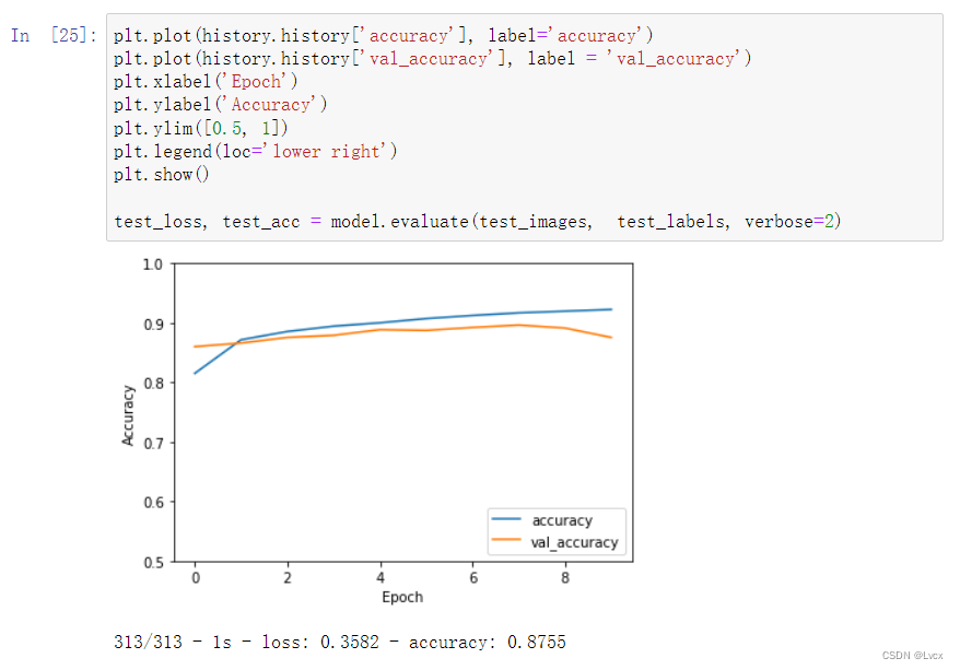
plt.plot(history.history['accuracy'], label='accuracy') plt.plot(history.history['val_accuracy'], label = 'val_accuracy') plt.xlabel('Epoch') plt.ylabel('Accuracy') plt.ylim([0.5, 1]) plt.legend(loc='lower right') plt.show() test_loss, test_acc = model.evaluate(test_images, test_labels, verbose=2)- 1
- 2
- 3
- 4
- 5
- 6
- 7
- 8
- 9
-
相关阅读:
164. 最大间距
[含文档+PPT+源码等]精品基于Uniapp+SSM实现的Android的校园新闻管理系统实现的App[包运行成功]计算机毕业设计Android项目源码
黑客技术(网络安全)自学2024
02. Springboot集成Flyway
SQL Server 安装后,服务器再改名,造成名称不一致,查询并修改数据库服务器真实名称
不使用canvas怎么实现一个刮刮卡效果?
vue2升级vue3:vue2 vue-i18n 升级到vue3搭配VueI18n v9
深度学习在蛋白质结构预测的新突破:AlphaFold、RoseTTAFold与ESMFold
linux下,如何查看一个文件的哈希值md5以及sha264
什么是Transformer架构的自注意力机制?
- 原文地址:https://blog.csdn.net/ungoing/article/details/126215733