【R语言】【2】绘图base和lattice和ggplot2库

前言

本来觉得r语言的library装起来很方便，要么是运行后有提示某个包没有，直接有install的选项，要么是用install.package(“包名”)也可以装上。问题是缺的包也太多了吧，好不容易装上gganimate，又提示已经被deprecated了。R语言在一两年前又有大更新，毕竟VSCode运行R.exe变成运行Python包的radian.exe了。能用的绘图函数可难找。

---

         \;\\\;\\\;

数据集mtcars

32辆汽车（1973-74款）的油耗和10个方面的汽车设计和性能

• mtcars$mpg ：每加仑油能跑多少英里
• mtcars$cyl ：气缸的个数
• mtcars$disp ：车的排量
• mtcars$hp ：总马力
• mtcars$drat ：后轴比
• mtcars$wt ：重量
• mtcars$qsec ：衡量启动加速能力
• mtcars$vs ：引擎类型
• mtcars$am ：传动方式，自动变速0、手动变速1
• mtcars$gear ：前进齿轮数
• mtcars$carb ：化油器个数

         \;\\\;\\\;

base

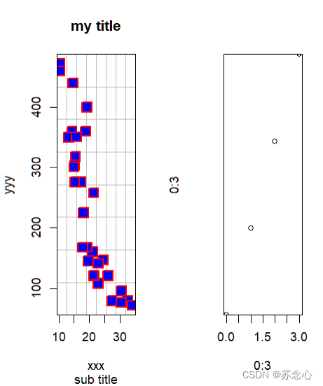
plot 散点图

#加载数据
#32辆汽车（1973-74款）的油耗和10个方面的汽车设计和性能
#data('mtcars')
# mtcars <- mtcars


#图为一行一列
# par(mfrow=c(1,1))

#图为一行两列
par(mfrow=c(1,2))

#散点图
plot(x=mtcars$mpg,y=mtcars$disp,
     type='p',     #散点图p,不显示n,折线图l,间断折线c
                   #散点+间断折线b,散点+连续折线o
                   #垂直于x轴h,楼梯s,反楼梯S
     main='my title',  #标题
     sub='sub title',  #副标题
     xlab='xxx',
     ylab='yyy',
     cex=2,        #点的大小
     lwd=2,        #边框线粗
     pch=22,       #点的形状,填充正方体22
     col='red',    #点的颜色
     bg='blue',    #填充颜色
     panel.first = grid(8,8,col='grey',lty=1),
     frame.plot = T
     )

plot(0:3,0:3,
     ann=T,        #正常显示标题和坐标轴标签T，不显示F
     axes=T,       #不显示边框F，显示边框T
     
     xaxs='r',     #x轴延伸r
     yaxs='i',     #y轴不延伸i
     
     xaxt='s',     #x轴数据显示s
     yaxt='n',     #y轴数据不显示n
     
     # log='xy'      #xy都取对数
     )

#额外的橙色网格
# grid(col='orange',lty=1)

1
2
3
4
5
6
7
8
9
10
11
12
13
14
15
16
17
18
19
20
21
22
23
24
25
26
27
28
29
30
31
32
33
34
35
36
37
38
39
40
41
42
43
44
45
46

         \;\\\;\\\;

pch点的形状

         \;\\\;\\\;

hist 直方图

#正太分布100个，平均30，方差3
a <- rnorm(100,30,3)

#1x2
par(mfrow=c(1,2))

hist(a,
     main="(1)",
     xlab="xxx",
     ylab="yyy",
     xlim=c(10,50),   #x轴范围
     ylim=c(0,25),    #y轴范围
     col='red',       #填充色
     # border='blue',   #边框色
     # breaks=30,       #分组组数
     breaks=function(x)length(x)/10,   #分组组数
     freq=T           #T显示频数，F显示概率密度
     )

hist(a,
     main="(2)",
     axes=T,          #显示坐标轴
     breaks=seq(10,50,by=4),   #(10,14) (14,18) ...
     freq=F,         
     #probability参数和freq意思相反，就忽略这个参数了
     label=T          #标签显示
     )
1
2
3
4
5
6
7
8
9
10
11
12
13
14
15
16
17
18
19
20
21
22
23
24
25
26
27

         \;\\\;\\\;

breaks意思

breaks的意思，是建议的分组组数

• 为一个 数 时，就是规定了横坐标自变量的个数
• 为一个矢量 c() 或者序列 seq() 时，向量的元素值就是各个横坐标自变量
• 为一个函数 function() 时，函数值表示分组组数，x表示总的数据个数，因此这里的breaks绘图前就固定不变了

         \;\\\;\\\;

boxplot 箱形图

以自变量进行分组，每个分组的因变量有一个范围，因此有最大、最小、平均、1/4和3/4，这些数据组成了一个个箱子

另外，限定了ylim值范围后，会出现异常值，为圆圈$\stackrel{◯}{}$，在min下面或者max上面

age <-    c(12 ,13 ,14 ,13 ,12 ,14 ,12 ,13 ,14 ,15 ,16)
height <- c(157,162,160,162,165,172,170,162,159,175,179)

#有大小写之分，因为都是字符串
gender <- c('f','f','m','m','f','f','f','f','m','f','m')

#分组数据
#max.
#3rd Qu.  所有数值由小到大排列后第75%的数字
#mean
#1st Qu.  所有数值由小到大排列后第25%的数字
#min.

par(mfrow=c(1,2))

boxplot(
  height~age,
  col='lightgray'
)


boxplot(
  height~gender,
  col=c('green','blue')
  # width=c(1,2),   #宽度设置
  # notch=T,        #有凹口
  # horizontal = T  #水平绘制
)
1
2
3
4
5
6
7
8
9
10
11
12
13
14
15
16
17
18
19
20
21
22
23
24
25
26
27
28

         \;\\\;\\\;

lattice

xyplot 散点图

library(lattice)

g <- factor(
  mtcars$gear,
  levels=c(3,4,5),
  labels=c("3 gears","4 gears",'5 gears')
)

xyplot(
  mtcars$mpg ~ mtcars$wt | mtcars$cyl * g,
  main="title"
  # xlab='xxx',
  # ylab='yyy'
)
1
2
3
4
5
6
7
8
9
10
11
12
13
14

         \;\\\;\\\;

histogram 直方图

library(lattice)

h <- c(21,20,27, 25,25,24,30,27, 27, 28, 29,27, 25, 25, 28, 26, 28, 26, 28, 31, 30, 26, 26)

histogram(
  h,
  col='yellow',
  border='red'
)
1
2
3
4
5
6
7
8
9

         \;\\\;\\\;

bwplot 箱型图

library(lattice)

age <-    c(12 ,13 ,14 ,13 ,12 ,14 ,12 ,13 ,14 ,15 ,16)
weight <- c( 50,52 , 54,60 , 66, 49, 52, 55,55 , 54, 60)
  
bwplot(
  weight~age,
  horizontal=F,    #是否横向显示
  cex=2,           #点的大小
  pch=16,          #点的形状
  box.ratio=0.9,
  box.width=0.9
)
1
2
3
4
5
6
7
8
9
10
11
12
13

         \;\\\;\\\;

ggplot2

ggplot + geom_point 散点图

library(ggplot2)


gear <- as.factor(mtcars$gear)

ggplot(mtcars,
       aes(mtcars$wt,mtcars$mpg,fill=gear)) + #aes()映射 fill填充颜色
  geom_point(
    size=6,shape=22     #shape和pch一样，是点的形状
  )
1
2
3
4
5
6
7
8
9
10

         \;\\\;\\\;

ggplot + geom_bar 直方图

library(ggplot2)
library(tidyverse)


data.frame(
  x=c('A','B','C'),
  y=c(rep('negative',7) ,rep('positive',11)  )
) %>% 
  ggplot(
    aes(x=x,fill=y)
  ) +
  geom_bar() +  #只需要x
  annotate(
    'text',
    x=1,y=3,
    label='50%',
    colour='white',
    fontface='bold')+
  annotate(
    'text',
    x=2,y=4,
    label='67%',
    colour='white',
    fontface='bold' )+
  annotate(
    'text',
    x=3,y=4,
    label='67%',
    colour='white',
    fontface='bold' )
1
2
3
4
5
6
7
8
9
10
11
12
13
14
15
16
17
18
19
20
21
22
23
24
25
26
27
28
29
30

library(ggplot2)
library(tidyverse)


ggplot(
  diamonds,
  aes(price,fill=cut)
)+
  geom_bar(stat='bin')  #只需要x
1
2
3
4
5
6
7
8
9

         \;\\\;\\\;

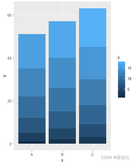
ggplot + geom_col 直方图

library(ggplot2)
library(tidyverse)


data.frame(
  x=c('A','B','C'),
  y=1:18
) %>% 
  ggplot(
    aes(x=x,y=y,fill=y)
  )+
  geom_col() #需要xy
1
2
3
4
5
6
7
8
9
10
11
12

         \;\\\;\\\;

ggplot + geom_histogram 直方图

library(ggplot2)
library(tidyverse)

age <-    c(12,13 ,13 ,13 ,13 ,12 ,14 ,12 ,16 ,14 ,15 ,16)

weight <- c(51, 50,52 , 55,55 , 66, 49, 52, 55,55 , 54, 60)

data.frame(
  x=age,
  y=weight
) %>%
  ggplot(
    aes(x=x,fill=y)
  ) +
  geom_histogram(
    breaks=seq(as.factor(weight)) + xlim(45,70)
                 )
1
2
3
4
5
6
7
8
9
10
11
12
13
14
15
16
17

         \;\\\;\\\;

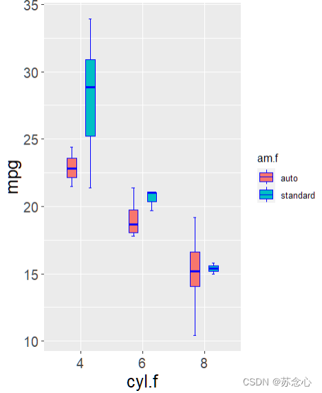
ggplot + geom_boxplot 箱型图

library(ggplot2)



cyl.f <- factor(
  mtcars$cyl,levels=c(4,6,8),labels=c('4','6','8')
)

am.f <- factor(
  mtcars$am,levels=c(0,1),labels=c('auto','standard')
)



ggplot(
  mtcars,
  aes(cyl.f,mpg)
) +
  stat_boxplot( 
    aes(fill=am.f),                       #
    geom='errorbar',                      #
    width=0.1,                            #
    size=0.5,                             #
    position=position_dodge(0.6),         #
    color='blue'                          #
  ) +
  geom_boxplot(
    aes(fill=am.f),                       #
    position=position_dodge(0.6),         #
    size=0.5,                             #
    width=0.3,                            #
    color='blue',                         #
    outlier.color = 'blue',               #
    outlier.fill = 'red',                 #
    outlier.shape = 19,                   #
    outlier.size = 1.5,                   #
    outlier.stroke = 0.5,                 #
    outlier.alpha = 45,                   #
    notch=F,                              #无凹口
    notchwidth = 0.5                      #
  )+
  theme(
    axis.title = element_text(size=18),   #坐标轴字体大小
    axis.text = element_text(size=14)     #坐标轴字体大小
  ) 

1
2
3
4
5
6
7
8
9
10
11
12
13
14
15
16
17
18
19
20
21
22
23
24
25
26
27
28
29
30
31
32
33
34
35
36
37
38
39
40
41
42
43
44
45
46

         \;\\\;\\\;

参考：
《R语言编程与绘图基础》
R语言 柱状图 geom_col 与 geom_bar 与geom_histogram（直方图）
R语言绘图基础篇-箱型图