Information Theory, 1948

• Shannon, Claude Elwood. “A mathematical theory of communication.” ACM SIGMOBILE mobile computing and communications review 5.1 (2001): 3-55.

Entropy (熵)

Information

• 考虑一个离散随机变量 $X$，当观测到它的一个具体值 $x$ 时，我们能得到多少信息呢？信息量可以被理解为 “degree of surprise”，也就是说，一个不太可能发生的事件带来的信息量比经常发生的事件带来的信息量更多，一个必然会发生的事件则不会带来任何信息，因此，(1) 信息量 $h(x)$ 是 $p(x)$ 的减函数。同时，如果事件 $x,y$ 相互独立 ($p(x,y)=p(x)p(y)$)，则同时观察到 $x,y$ 带来的信息量为分别观察到 $x,y$ 带来的信息量之和相同，也就是 (2) $h(x,y)=h(x)+h(y)$. 由此可得信息量 $h(x)$ 的形式如下：
  其中，$h(x)\ge 0$，对数函数的底数是任意的，当底数为 2 时，信息量的单位为 bits，当底数为 $e$ 时，信息量的单位为 nats

Entropy

• 假设发射者向接收者传输离散随机变量的值，则传输过程中的平均信息量为 $h(x)$ 取期望的形式：
  其中，$H[x]$ 即为随机变量 $x$ 的熵。由于 ${\lim }_{p\to 0}p{\log }_{2}p=0$，因此当 $p(x)=0$ 时取 $p(x){\log }_{2}p(x)=0$，不可能发生的事件不会带来任何信息量 (熵是关于 $X$ 概率分布的凹函数，因此 $H[x]$ 也可以被记作 $H[p]$)
• 一个随机变量的熵越大，意味着不确定性越大，那么也就是说，该随机变量包含的信息量越大，也表示平均意义上对随机变量的编码长度

---

Entropy in bits

• (1) 考虑一个离散随机变量 $x\in \mathcal{X}$ 服从均匀分布，则传输 $x$ 的值时，需要的编码长度为 ${\log }_2|\mathcal{X}|$，也就是底数为 2 时 $X$ 的熵
• (2) 再考虑如下例子。假设一个离散随机变量有 8 种状态 { a , b , c , d , e , f , g , h } \{a, b, c, d, e, f, g, h\} {a,b,c,d,e,f,g,h}，它们的概率分别为 $(1/2,1/4,1/8,1/16,1/64,1/64,1/64,1/64)$，如果要高效地对其进行传输，可以利用哈夫曼编码得到每种状态的最优编码 $0$, $10$, $110$, $1110$, $111100$, $111101$, $111110$, $111111$，最优编码的平均编码长度为
  正好等于随机变量的熵：
  
• (3) noiseless coding theorem (Shannon, 1948) 指出，熵是传输随机变量需要的平均比特数的下界

Entropy in physics
熵的概念最早其实可以追溯到物理学中。在物理学中，熵就表示混乱程度。假设有 $N$ 个相同物体被放在若干 bins 中，其中 $i$-th bin 中放 $n_i$ 个物体，则分配方案的数量为
熵被定义为 $W$ 的对数形式再加上一个缩放因子的形式
当 $N\to \infty$ 且 $n_i/N$ 固定时，使用 Stirling’s approximation 可以得到
将其代入 $H$ 的表达式可得
H = 1 N ( N ln ⁡ N − N − ∑ i ( n i ln ⁡ n i − n i ) ) = 1 N ( N ln ⁡ N − ∑ i n i ln ⁡ n i ) = ∑ i ( n i N ) ln ⁡ N − ∑ i ( n i N ) ln ⁡ n i

H=1N(Nln⁡N−N−∑i(niln⁡ni−ni))=1N(Nln⁡N−∑iniln⁡ni)=∑i(niN)ln⁡N−∑i(niN)ln⁡ni" role="presentation" style="position: relative;">H=1N(NlnN−N−∑i(nilnni−ni))=1N(NlnN−∑inilnni)=∑i(niN)lnN−∑i(niN)lnni$$\begin{array}{rl}H& =\frac{1}{N}(N\ln N-N-\sum _i(n_i\ln n_i-n_i))\\ & =\frac{1}{N}(N\ln N-\sum _i{n}_i\ln n_i)\\ & =\sum _i\left(\frac{n_i}{N}\right)\ln N-\sum _i\left(\frac{n_i}{N}\right)\ln n_i\end{array}$$

H​=N1​(NlnN−N−i∑​(ni​lnni​−ni​))=N1​(NlnN−i∑​ni​lnni​)=i∑​(Nni​​)lnN−i∑​(Nni​​)lnni​​因此，

Properties

• (1) 概率分布越尖锐，熵越小；概率分布越平坦，熵越大。当 $X$ 服从均匀分布时熵最大，$H[X]=\ln |\mathcal{X}|$，其中 $\mathcal{X}$ 为采样空间；当 $X$ 只能取 1 个值时 ($p_i=1,p_{j\ne i}=0$) 熵最小，$H[X]=0$
  $$0\le H(X)\le \ln |\mathcal{X}|$$证明：下面求熵的最大值。求熵的最大值可以转化为求熵的负数的最小值，这就转化为了一个凸优化问题：
  $$\begin{gathered} \min \sum _{i}p(x_i)\ln p(x_i) \\ s.t.\sum _{i}p(x_i)=1,0\le p(x_i)\le 1 \end{gathered}$$暂时忽略第 2 个约束条件，可以写出拉格朗日函数：
  $$L(p(x_i),\lambda )=\sum _{i}p(x_i)\ln p(x_i)+\lambda (\sum _{i}p(x_i)-1)$$令其偏导为 0：
  $$\begin{gathered} \frac{\partial L}{\partial p(x_i)}=1+\ln p(x_i)+\lambda =0 \\ \frac{\partial L}{\partial \lambda }=\sum _{i}p(x_i)-1=0 \end{gathered}$$因此有
  $$\begin{gathered} p(x_1)=p(x_2)=...=p(x_{|\mathcal{X}|})=\frac{1}{|\mathcal{X}|} \\ H[X]=\ln |\mathcal{X}| \end{gathered}$$该解满足第 2 个约束条件 $0\le p(x_i)\le 1$，是一个可行解
  

Differential entropy (微分熵)

• 熵的定义可以被推广到连续随机变量的情况。考虑将 $\mathcal{X}$ 分为若干个宽为 $\Delta$ 的 bins，对于 $i$-th bin，存在 $x_i$ 使得
  因此我们可以把 $i$-th bin 内的值都替换为 $x_i$ 从而将连续概率分布量化为离散概率分布，它的熵为
  其中，第 2 项 $-\ln \Delta$ 在 $\Delta \to 0$ 时发散，这说明精准表示一个连续变量需要大量 bits
• 我们先忽略第 2 项 $-\ln \Delta$ 并且考虑 $\Delta \to 0$ 的情况，此时有
  其中，等式右侧的项即为微分熵. 对于多元连续随机变量 $\mathbf{x}$ (a vector)，微分熵为
  

---

Maximum entropy configuration for a continuous variable - Gaussian Distribution

• 下面求微分熵的最大值。该问题是一个条件优化问题，$p(x)$ 满足如下约束：
  可以用拉格朗日乘子法转化为无条件约束的优化问题：
  
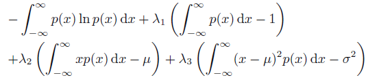
• 上式是一个有关概率分布 $p(x)$ 的泛函，将其整理一下可得
  F [ p ( x ) ] = ∫ − ∞ ∞ [ − p ( x ) ln ⁡ p ( x ) + λ 1 p ( x ) + λ 2 x p ( x ) + λ 3 ( x − μ ) 2 p ( x ) ] d x + ( − λ 1 − λ 2 μ − λ 3 σ 2 ) = ∫ − ∞ ∞ G ( p ( x ) , x ) d x + C
  F[p(x)]=∫−∞∞[−p(x)ln⁡p(x)+λ1p(x)+λ2xp(x)+λ3(x−μ)2p(x)]dx+(−λ1−λ2μ−λ3σ2)=∫−∞∞G(p(x),x)dx+C" role="presentation" style="position: relative;">F[p(x)]=∫∞−∞[−p(x)lnp(x)+λ1p(x)+λ2xp(x)+λ3(x−μ)2p(x)]dx+(−λ1−λ2μ−λ3σ2)=∫∞−∞G(p(x),x)dx+C$$\begin{array}{rl}F[p(x)]& ={\int }_{-\mathrm{\infty }}^{\mathrm{\infty }}\left[-p(x)\ln p(x)+{\lambda }_{1}p(x)+{\lambda }_{2}xp(x)+{\lambda }_3(x-\mu {)}^{2}p(x)\right]dx+(-{\lambda }_1-{\lambda }_2\mu -{\lambda }_3{\sigma }^2)\\ & ={\int }_{-\mathrm{\infty }}^{\mathrm{\infty }}G(p(x),x)dx+C\end{array}$$
  F[p(x)]​=∫−∞∞​[−p(x)lnp(x)+λ1​p(x)+λ2​xp(x)+λ3​(x−μ)2p(x)]dx+(−λ1​−λ2​μ−λ3​σ2)=∫−∞∞​G(p(x),x)dx+C​由欧拉-拉格朗日方程可知，当 $p(x)$ 使得 $F[p(x)]$ 取极值时，对任意 $x$ 有
  δ F δ p ( x ) = ∂ G ∂ p − d d x ( ∂ G ∂ p ′ ) = ∂ G ∂ p = − 1 − ln ⁡ p ( x ) + λ 1 + λ 2 x + λ 3 ( x − μ ) 2 = 0
  δFδp(x)=∂G∂p−ddx(∂G∂p′)=∂G∂p=−1−ln⁡p(x)+λ1+λ2x+λ3(x−μ)2=0" role="presentation" style="position: relative;">δFδp(x)=∂G∂p−ddx(∂G∂p′)=∂G∂p=−1−lnp(x)+λ1+λ2x+λ3(x−μ)2=0$$\begin{array}{rl}\frac{\delta F}{\delta p(x)}& =\frac{\mathrm{\partial }G}{\mathrm{\partial }p}-\frac{d}{dx}\left(\frac{\mathrm{\partial }G}{\mathrm{\partial }{p}^{\prime }}\right)=\frac{\mathrm{\partial }G}{\mathrm{\partial }p}\\ & =-1-\ln p(x)+{\lambda }_1+{\lambda }_{2}x+{\lambda }_3(x-\mu {)}^2\\ & =0\end{array}$$
  δp(x)δF​​=∂p∂G​−dxd​(∂p′∂G​)=∂p∂G​=−1−lnp(x)+λ1​+λ2​x+λ3​(x−μ)2=0​因此，
  将其带入 3 个约束式就可以得到拉格朗日乘子 ${\lambda }_1,{\lambda }_2,{\lambda }_3$ 的值 (过程比较复杂，可以参考 Exercise 1.34)，最终可以得到
  也就是说，正态分布可以使得微分熵最大 (在上述优化过程中，我们并没有约束 $p(x)\ge 0$，但由于求出来的 $p(x)$ 满足该约束，因此非负的约束项可以不加)，将 $p(x)$ 代入微分熵的表达式可得
  H [ x ] = − ∫ p ( x ) ln ⁡ p ( x ) d x = − ∫ p ( x ) ln ⁡ { 1 2 π σ 2 } d x − ∫ p ( x ) { − ( x − μ ) 2 2 σ 2 } d x = − ln ⁡ { 1 2 π σ 2 } + σ 2 2 σ 2 = 1 2 { 1 + ln ⁡ ( 2 π σ 2 ) }
  H[x]=−∫p(x)ln⁡p(x)dx=−∫p(x)ln⁡{12πσ2}dx−∫p(x){−(x−μ)22σ2}dx=−ln⁡{12πσ2}+σ22σ2=12{1+ln⁡(2πσ2)}" role="presentation" style="position: relative;">H[x]=−∫p(x)lnp(x)dx=−∫p(x)ln{12πσ2}dx−∫p(x){−(x−μ)22σ2}dx=−ln{12πσ2}+σ22σ2=12{1+ln(2πσ2)}$$\begin{array}{rl}H[x]& =-\int p(x)\ln p(x)dx\\ & =-\int p(x)\ln \left\{\frac{1}{2\pi {\sigma }^2}\right\}dx-\int p(x)\left\{-\frac{(x-\mu {)}^2}{2{\sigma }^2}\right\}dx\\ & =-\ln \left\{\frac{1}{2\pi {\sigma }^2}\right\}+\frac{{\sigma }^2}{2{\sigma }^2}\\ & =\frac{1}{2}\left\{1+\ln \left(2\pi {\sigma }^2\right)\right\}\end{array}$$
  H[x]​=−∫p(x)lnp(x)dx=−∫p(x)ln{2πσ21​}dx−∫p(x){−2σ2(x−μ)2​}dx=−ln{2πσ21​}+2σ2σ2​=21​{1+ln(2πσ2)}​其中，${\sigma }^2$ 越大，微分熵越大，并且 $H[x]$ 可能取负值

Joint Entropy and Conditional Entropy (联合熵，条件熵)

Conditional Entropy

• 已知 $x$ 的情况下观察到 $y$ 的值带来的额外信息量为 $-\ln p(y|x)$. 假如我们从联合概率 $p(x,y)$ 中抽样 $(x,y)$，则已知 $x$ 时观察到 $y$ 带来的平均额外信息量为
  上式即为给定 $X$ 时 $Y$ 的条件熵，并且有 $H[Y|X]\le H[Y]$
• 条件熵也可写为下式：
  H [ Y ∣ X ] = − ∬ p ( y , x ) ln ⁡ p ( y ∣ x ) d y d x = − ∫ p ( x ) ∫ p ( y ∣ x ) ln ⁡ p ( y ∣ x ) d y d x = ∫ p ( x ) H [ Y ∣ x ] d x
  H[Y|X]=−∬p(y,x)ln⁡p(y|x)dydx=−∫p(x)∫p(y|x)ln⁡p(y|x)dydx=∫p(x)H[Y|x]dx" role="presentation" style="position: relative;">H[Y|X]=−∬p(y,x)lnp(y|x)dydx=−∫p(x)∫p(y|x)lnp(y|x)dydx=∫p(x)H[Y|x]dx$$\begin{array}{rl}H[Y|X]& =-\iint p(y,x)\ln p(y|x)dydx\\ & =-\int p(x)\int p(y|x)\ln p(y|x)dydx\\ & =\int p(x)H[Y|x]dx\end{array}$$
  H[Y∣X]​=−∬p(y,x)lnp(y∣x)dydx=−∫p(x)∫p(y∣x)lnp(y∣x)dydx=∫p(x)H[Y∣x]dx​Zero conditional entropy: 由上式可知，当 $H[Y|X]=0$ 时，对所有 $x$ 都有 $H[Y|x]=0$，也就是当 $x$ 固定时，$y$ 只能取某一个定值

---

Joint Entropy

$$H[x,y]=-\iint p(x,y)\ln p(x,y)dydx$$

• $H[x,x]=H[x]$
• $H[x,y]=H[y,x]$

---

Chain Rule

Relative entropy / KL divergence / KL distance (相对熵, KL 散度, KL 距离)

• 假如有一个未知的概率分布 $p(x)$，我们用另一个概率分布 $q(x)$ 来近似 $p(x)$. 如果我们在传输 $x$ 的值时使用 $q(x)$ 构筑编码方式，则与实际使用 $p(x)$ 构筑编码方式相比，需要的平均额外信息量 (in nats) 为
  上式即为相对熵 / KL 散度 (KL divergence is a measure of the inefficiency of assuming that the distribution is $q$ when the true distribution is $p$. e.g. if we knew the true distribution $p$ of the random variable, we could construct a code with average description length $H(p)$. If, instead, we used the code for a distribution $q$, we would need $H(p)+KL(p\Vert q)$ bits on the average to describe the random variable. i.e.
  $H(q)=H(p)+KL(p\Vert q)$)，它可以用来度量两个概率分布之间的距离 (两个概率分布的采样空间必须相同)。注意到，KL 散度是非对称量，即 $KL(p\Vert q)\ne KL(q\Vert p)$
• 注意到，$0\log \frac{0}{0}=0,0\log \frac{0}{q}=0,p\log \frac{p}{0}=\infty$，因此如果存在 $x\in \mathcal{X}$ 使得 $p(x)>0$ 但 $q(x)=0$, 则 $KL(p\Vert q)=\infty$

---

Gibbs’s inequality

K L ( p ∥ q ) ≥ 0 with equality if and  only if  p ( x ) = q ( x )  for all  x

with equality if and ​KL(p∥q)≥0only if p(x)=q(x) for all x​

Proof

• Jensen’s inequality：凸函数：
  其中，$0\le \lambda \le 1$
  由数学归纳法可知，凸函数 $f(x)$ 满足
  其中，${\lambda }_i\ge 0$，${\sum }_i{\lambda }_i=1$. 上式即为 Jensen’s inequality，证明如下：
  f ( ∑ m = 1 M + 1 λ m x m ) = f ( λ M + 1 x M + 1 + ( 1 − λ M + 1 ) ∑ m = 1 M λ m 1 − λ M + 1 x m ) ≤ λ M + 1 f ( x M + 1 ) + ( 1 − λ M + 1 ) f ( ∑ m = 1 M λ m 1 − λ M + 1 x m ) ≤ λ M + 1 f ( x M + 1 ) + ( 1 − λ M + 1 ) ∑ m = 1 M λ m 1 − λ M + 1 f ( x m ) ≤ ∑ m = 1 M + 1 λ m f ( x m )
  f(∑m=1M+1λmxm)=f(λM+1xM+1+(1−λM+1)∑m=1Mλm1−λM+1xm)≤λM+1f(xM+1)+(1−λM+1)f(∑m=1Mλm1−λM+1xm)≤λM+1f(xM+1)+(1−λM+1)∑m=1Mλm1−λM+1f(xm)≤∑m=1M+1λmf(xm)" role="presentation" style="position: relative;">f(∑m=1M+1λmxm)=f(λM+1xM+1+(1−λM+1)∑m=1Mλm1−λM+1xm)≤λM+1f(xM+1)+(1−λM+1)f(∑m=1Mλm1−λM+1xm)≤λM+1f(xM+1)+(1−λM+1)∑m=1Mλm1−λM+1f(xm)≤∑m=1M+1λmf(xm)$$\begin{array}{rl}f\left(\sum _{m=1}^{M+1}{\lambda }_m{x}_m\right)& =f\left({\lambda }_{M+1}{x}_{M+1}+\left(1-{\lambda }_{M+1}\right)\sum _{m=1}^M\frac{{\lambda }_m}{1-{\lambda }_{M+1}}{x}_m\right)\\ & \le {\lambda }_{M+1}f\left(x_{M+1}\right)+\left(1-{\lambda }_{M+1}\right)f\left(\sum _{m=1}^M\frac{{\lambda }_m}{1-{\lambda }_{M+1}}{x}_m\right)\\ & \le {\lambda }_{M+1}f\left(x_{M+1}\right)+\left(1-{\lambda }_{M+1}\right)\sum _{m=1}^M\frac{{\lambda }_m}{1-{\lambda }_{M+1}}f\left(x_m\right)\\ & \le \sum _{m=1}^{M+1}{\lambda }_{m}f\left(x_m\right)\end{array}$$
  f(m=1∑M+1​λm​xm​)​=f(λM+1​xM+1​+(1−λM+1​)m=1∑M​1−λM+1​λm​​xm​)≤λM+1​f(xM+1​)+(1−λM+1​)f(m=1∑M​1−λM+1​λm​​xm​)≤λM+1​f(xM+1​)+(1−λM+1​)m=1∑M​1−λM+1​λm​​f(xm​)≤m=1∑M+1​λm​f(xm​)​如果将 ${\lambda }_i$ 视为离散随机变量 $z$ 的概率分布，即 ${\lambda }_i=p(z=z_i)$，$x_i=\xi (z_i)$，则 Jensen 不等式可以写为
  $$f({\mathbb{E}}_z[\xi (z)])\le {\mathbb{E}}_z[f(\xi (z))]$$其中，$f$ 为凸函数，$\xi$ 为任意函数。如果 $f$ 为严格凸函数，则当且仅当 “$\xi (z)$ is constant with probability one or $almost$ $surely$” 时等号成立 ($almost$ $surely$ 表明可能存在例外，但例外发生的概率为 0)，此时有 $\xi (z)={\xi }_0$ (on the range of $z$ almost everywhere)，因此 ${\mathbb{E}}_z[\xi (z)]={\xi }_0$，Jensen 不等式的左右均为 $f({\xi }_0)$
  并且 Jensen 不等式也可以推广到连续随机变量
  
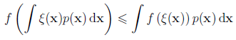
• 由于 $-\ln x$ 为凸函数，将 Jensen 不等式代入 KL 散度公式可知
  $$\mathrm{KL}(p\Vert q)=-\int p(\mathrm{x})\ln \left\{\frac{q(\mathrm{x})}{p(\mathrm{x})}\right\}\mathrm{dx}⩾-\ln \int p(\mathrm{x})\frac{q(\mathrm{x})}{p(\mathrm{x})}\mathrm{dx}\ge 0$$其中最后 $-\ln \int p(\mathrm{x})\frac{q(\mathrm{x})}{p(\mathrm{x})}\mathrm{dx}\ge 0$ 是因为 $-\ln \int p(\mathrm{x})\frac{q(\mathrm{x})}{p(\mathrm{x})}\mathrm{dx}$ 中，如果 $p(x)=0$ 则 $p(x)\frac{q(x)}{p(x)}=0$，因此最后得出的 $\int p(\mathrm{x})\frac{q(\mathrm{x})}{p(\mathrm{x})}\mathrm{dx}$ 可能少掉某些 $q(x)$ 项，使得最终的和小于 1. 由于 $-\ln x$ 为严格凸函数，因此当且仅当 $p(x)=q(x)$ almost everywhere 时 $\mathrm{KL}(p\Vert q)=0$

---

KL divergence for density estimation

• 假设我们想要建模的数据服从一个未知分布 $p(x)$，我们用一个参数化的分布 $q(x|\theta )$ 去近似 $p(x)$，此时就通过最小化 $KL(p\Vert q)$ 来优化参数 $\theta$. 但我们并不知道 $p(x)$ 的具体值，只能从中采样，因此期望项需要用蒙特卡洛法来近似，也就是从 $p(x)$ 中采样出 $N$ 个样本点来近似地计算 KL 散度：
  K L ( p ∥ q ) ≃ 1 N ∑ n = 1 N { − ln ⁡ q ( x n ∣ θ ) + ln ⁡ p ( x n ) } \mathrm{KL}(p \| q) \simeq \frac{1}{N}\sum_{n=1}^{N}\left\{-\ln q\left(\mathrm{x}_{n} \mid \boldsymbol{\theta}\right)+\ln p\left(\mathrm{x}_{n}\right)\right\} KL(p∥q)≃N1​n=1∑N​{−lnq(xn​∣θ)+lnp(xn​)}第 2 项为定值可以忽略，因此最小化 KL 散度等价于最大化对数似然

---

Cross entropy loss

• 在 ML 的分类问题中，样本 $i$ 的标签 $t_i$ 可以被表示为 one-hot vector，该向量可以被看作是一个离散概率分布 $p_i(z)$. 模型经过 softmax 的预测结果也可以被看作一个离散概率分布 $q_i(z|\theta )$，我们想要让 $p_i(z)$ 和 $q_i(z|\theta )$ 之间的 KL 散度尽量小：
  min ⁡ θ K L ( p i ( z ) ∥ q i ( z ∣ θ ) ) = min ⁡ θ E z ∼ p i ( z ) [ ln ⁡ p i ( z ) q i ( z ∣ θ ) ] = min ⁡ θ − E z ∼ p i ( z ) [ ln ⁡ q i ( z ∣ θ ) ]
  minθKL(pi(z)‖qi(z|θ))=minθEz∼pi(z)[ln⁡pi(z)qi(z|θ)]=minθ−Ez∼pi(z)[ln⁡qi(z|θ)]" role="presentation" style="position: relative;">minθKL(pi(z)∥qi(z|θ))=minθEz∼pi(z)[lnpi(z)qi(z|θ)]=minθ−Ez∼pi(z)[lnqi(z|θ)]$$\begin{array}{rl}\underset{\theta }{min}KL(p_i(z)\Vert q_i(z|\theta ))& =\underset{\theta }{min}{\mathbb{E}}_{z\sim p_i(z)}\left[\ln \frac{p_i(z)}{q_i(z|\theta )}\right]\\ & =\underset{\theta }{min}-{\mathbb{E}}_{z\sim p_i(z)}\left[\ln q_i(z|\theta )\right]\end{array}$$
  θmin​KL(pi​(z)∥qi​(z∣θ))​=θmin​Ez∼pi​(z)​[lnqi​(z∣θ)pi​(z)​]=θmin​−Ez∼pi​(z)​[lnqi​(z∣θ)]​又因为 $p_i(z)$ 只在标签处概率值为 1 (i.e. $p_i(z)=1$, if $z=t_i$ else 0)，因此有
  min ⁡ θ K L ( p i ( z ) ∥ q i ( z ∣ θ ) ) = min ⁡ θ − ln ⁡ q i ( t i ∣ θ )
  minθKL(pi(z)‖qi(z|θ))=minθ−ln⁡qi(ti|θ)" role="presentation" style="position: relative;">minθKL(pi(z)∥qi(z|θ))=minθ−lnqi(ti|θ)$$\begin{array}{rl}\underset{\theta }{min}KL(p_i(z)\Vert q_i(z|\theta ))& =\underset{\theta }{min}-\ln q_i(t_i|\theta )\end{array}$$
  θmin​KL(pi​(z)∥qi​(z∣θ))​=θmin​−lnqi​(ti​∣θ)​样本 $i$ 的损失函数为
  $$L_i=-\ln q_i(t_i|\theta )$$上式即为交叉熵损失

Mutual information (互信息)

• 现在考虑随机变量 $x$, $y$，如果它们相互独立，则有 $p(x,y)=p(x)p(y)$，因此可以用如下的 KL 散度来衡量随机变量 $x$, $y$ 的独立程度：
  上式即为随机变量 $x$, $y$ 的互信息，可以看到，独立程度越低，互信息越大 (a measure of the amount of information one random variable contains about another)

---

Properties

• $I[x,y]\ge 0$；当且仅当 $x,y$ 独立时有
  $$I[x,y]=0$$
• $I[x,y]=I[y,x]$
• $I[x,x]=KL(p(x)\Vert p(x{)}^2)={\int }_{x}p(x)\ln \frac{1}{p(x)}dx=H[x]$. Entropy then becomes the self-information of a random variable.

---

Mutual Information and Entropy

• Mutual Information is the reduction in the uncertainty of one random variable due to the knowledge of the other.
  $$I[X,Y]=H[X]+H[Y]-H[X,Y]$$Proof sketch: e.g. To prove $I[X,Y]=H[X]+H[Y]-H[X,Y]$
  • (1)
    $$\log \frac{p(X,Y)}{p(X)p(Y)}=-\log p(X)-\log p(Y)+\log p(X,Y)$$
  • (2) Take expectation $E$ at both sides.
• For two random variables $X,Y$, if $X$ and $Y$ are independent, then
  $$H[X,Y]=H[X]+H[Y]$$

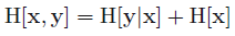
Chain rules for entropy, relative entropy, and mutual information

Chain Rule for Entropy

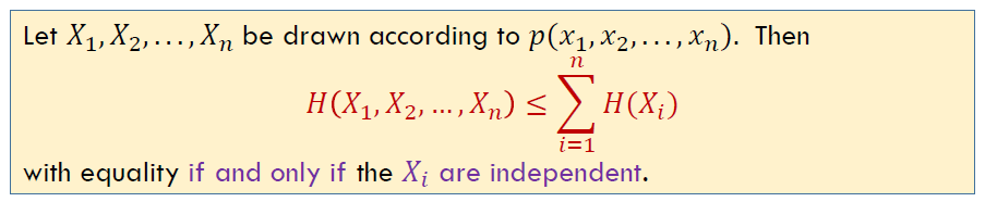
• The entropy of a collection of random variables is the sum of the conditional entropies.
  
  • If $X_1,...,X_n$ are independent,
    

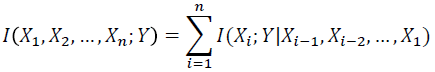
Proof

• (1) Fact $p(x_1,...,x_n)=p(x_1)p(x_2|x_1)...p(x_n|x_1,...,x_{n-1})$
• (2) Take $\log ()$ at each side
• (3) Take expectation $E$ at both sides: $E(X_1+X_2)=E(X_1)+E(X_2)$

---

Conditional mutual information

• We now define the conditional mutual information as the reduction in the uncertainty of $X$ due to knowledge of $Y$ when $Z$ is given.

• $I(X;Y|Z)\ge 0$ with equality if and only if $X$ and $Y$ are conditionally independent given $Z$

---

Chain rule for information

---

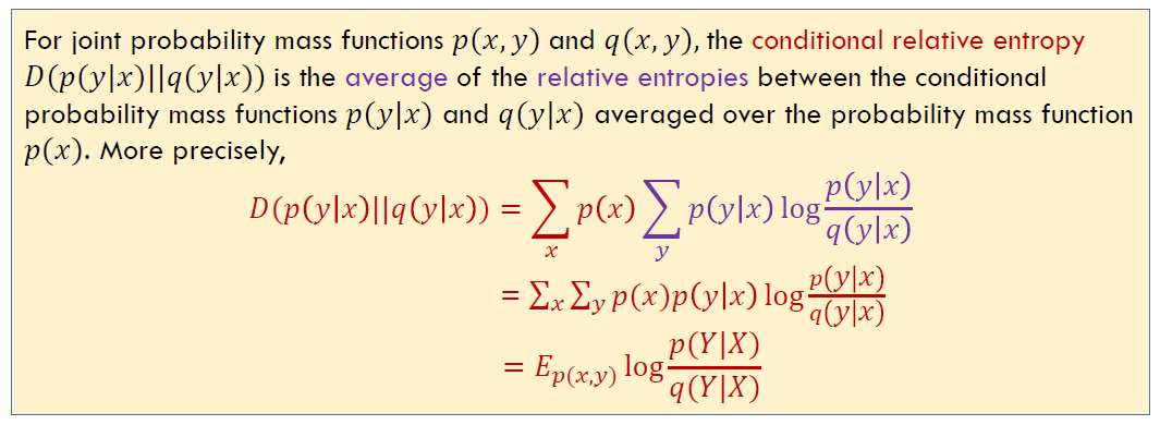
Conditional Relative Entropy

---

Chain rule for relative entropy

• Proof:
  

Information inequality (信息不等式)

Independence Bound on Entropy

• Proof: By chain rule for entropies,
  

References

• 上海交通大学程帆老师信息论课程
• Bishop, Christopher M., and Nasser M. Nasrabadi. Pattern recognition and machine learning. Vol. 4. No. 4. New York: springer, 2006.
• 【PRML】【模式识别和机器学习】【从零开始的公式推导】1.6 信息论
• Solution Manual For PRML
• More PRML Errata