前言
支持向量机是一类按监督学习方式对数据进行二元分类的广义线性分类器,其决策边界是对学习样本求解的最大边距超平面。SVM尝试寻找一个最优决策边界,使距离两个类别最近的样本最远。
SVM使用铰链损失函数计算经验风险并在求解系统中加入了正则化项以优化结构风险,是一个具有稀疏性和稳健性的分类器 。SVM可以通过核方法(kernel method)进行非线性分类,是常见的核学习(kernel learning)方法之一
SVM原理
-
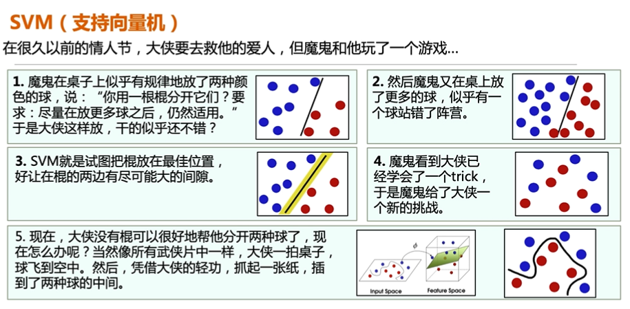
引入
-
直观理解
- 对数据进行分类,当超平面数据点‘间隔’越大,分类的确信度也越大。
- 我们上面用的棍子就是分类平面。
-
支持向量

- 我们可以看到决定分割面其实只有上面4个红色的点决定的,这四个点就叫做支持向量。
非线性SVM与核函数
如何变幻空间
对于非线性的数据我们是通过核函数把数据分为不同的平面在进行处理。

- 核函数
- 线性核函数:K(x,z) = x*z
- 多项式核函数:K(x,z) = (x*z+1)^p
- 高斯核函数:K(x,z) = exp()
- 混合核:K(x,z) = aK1(x,z)+(1-a)K2(x,z), 0<=a<1\
多分类处理应用
-
一对多法(OVR SVMs)
- 训练时依次把某个类别样本归为一类,其他剩余样本归为一类
- k个SVM:分类时将未知样本分类为具有最大分类函数值的那类
-
一对一法(OVO SVMs或者pairwise)
- 在任意两类样本之间设计一个SVM
- k(k-1)/2个SVM
- 当对一个未知样本进行分类时,最后得票最多的类别即为该未知样本的类。
-
层次SVM
- 层次分类法首先将所有类别分成两个子类,再将子类进一步划分成两个次级子类,如此循环,直到得到一个单独的类别为止。类似与二叉树分类。
优点
- 相对于其他分类算法不需要过多样本,并且由于SVM引入核函数,所以SVM可以处理高维样本。
- 结构风险最小,这种风险是指分类器对问题真实模型的逼近与问题真实解之间的累计误差。
- 非线性,是指SVM擅长应对样本数据线性不可分的情况,主要通过松弛变量(惩罚变量)和核函数技术来实现,这也是SVM的精髓所在。
开源包
LibSVM:https://www.csie.ntu.edu.tw/~cjlin/libsvm/
Liblinear:https://www.csie.ntu.edu.tw/~cjlin/liblinear/
数据集
数据集是使用sklearn包中的数据集。也可以下载下来方便使用。
百度网盘:
链接:https://pan.baidu.com/s/16H2xRXQItIY0hU0_wIAvZw
提取码:vq2i
SVM实现鸢尾花分类
- 代码
复制代码
- 1
- 2
- 3
- 4
- 5
- 6
- 7
- 8
- 9
- 10
- 11
- 12
- 13
- 14
- 15
- 16
- 17
- 18
- 19
- 20
- 21
- 22
- 23
- 24
- 25
- 26
- 27
- 28
- 29
- 30
- 31
- 32
- 33
- 34
- 35
- 36
- 37
- 38
- 39
- 40
- 41
- 42
- 43
- 44
- 45
- 46
- 47
- 48
- 49
- 50
- 51
- 52
- 53
- 54
- 55
- 56
- 57
- 58
- 59
- 60
- 61
- 62
- 63
- 64
- 65
- 66
- 67
- 68
- 69
- 70
- 71
- 72
- 73
- 74
- 75
- 76
- 77
- 78
- 79
- 80
- 81
- 82
- 83
- 84
- 85
- 86
- 87
- 88
- 89
- 90
- 91
- 92
- 93
- 94
- 95
- 96
er-hljs
## 数据集 sklearn中


import numpy as np

import matplotlib as mpl
import matplotlib.pyplot as plt
from matplotlib import colors

from sklearn import svm
from sklearn import model_selection


## 加载数据集

def iris_type(s):
    it = {b'Iris-setosa':0, b'Iris-versicolor':1, b'Iris-virginica':2}
    return it[s]


data = np.loadtxt('Iris-data/iris.data',dtype=float,delimiter=',',converters={4:iris_type})

x,y = np.split(data, (4, ), axis=1)

x = x[:,:2]
x_train,x_test, y_train, y_test = model_selection.train_test_split(x,y,random_state=1,test_size=0.2)


## 构建SVM分类器,训练函数

def classifier():
    clf = svm.SVC(C=0.8, kernel='linear', decision_function_shape='ovr')
    return clf

def train(clf, x_train, y_train):
    clf.fit(x_train, y_train.ravel())


clf = classifier()
train(clf,x_train,y_train)

## 初始化分类器,训练模型
def show_accuracy(a, b, tip):
    acc = a.ravel()==b.ravel()
    print('%s accracy:%.3f'%(tip, np.mean(acc)))

## 展示训练结果,及验证结果

def print_accracy(clf, x_train, y_train, x_test, y_test):
    print('training prediction:%.3f'%(clf.score(x_train, y_train)))
    print('test prediction:%.3f'%(clf.score(x_test, y_test)))

    show_accuracy(clf.predict(x_train),y_train, 'training data')
    show_accuracy(clf.predict(x_test), y_test, 'testing data')

    print('decision_function:\n',clf.decision_function(x_train)[:2])

print_accracy(clf, x_train, y_train, x_test, y_test)


def draw(clf, x):
    iris_feature = 'sepal length', 'sepal width', 'petal length', 'petal width'

    x1_min,x1_max = x[:,0].min(), x[:,0].max()
    x2_min,x2_max = x[:,1].min(), x[:,1].max()

    x1, x2 = np.mgrid[x1_min:x1_max:200j, x2_min:x2_max:200j]

    grid_test = np.stack((x1.flat, x2.flat), axis=1)
    print('grid_test:\n',grid_test[:2])

    z = clf.decision_function(grid_test)
    print('the distance:',z[:2])

    grid_hat = clf.predict(grid_test)
    print(grid_hat[:2])


    grid_hat = grid_hat.reshape(x1.shape)
    cm_light = mpl.colors.ListedColormap(['#A0FFA0', '#FFA0A0', '#A0A0FF'])
    cm_dark = mpl.colors.ListedColormap(['g', 'b', 'r'])

    plt.pcolormesh(x1, x2, grid_hat, cmap=cm_light)
    plt.scatter(x[:,0], x[:, 1],c=np.squeeze(y), edgecolors='k', s=50, cmap=cm_dark)
    plt.scatter(x_test[:,0],x_test[:,1], s=120, facecolor='none', zorder=10)
    plt.xlabel(iris_feature[0])
    plt.ylabel(iris_feature[1])
    plt.xlim(x1_min, x1_max)
    plt.ylim(x2_min, x2_max)
    plt.title('Iris data classification via SVM')
    plt.grid()
    plt.show()

draw(clf, x)
折叠
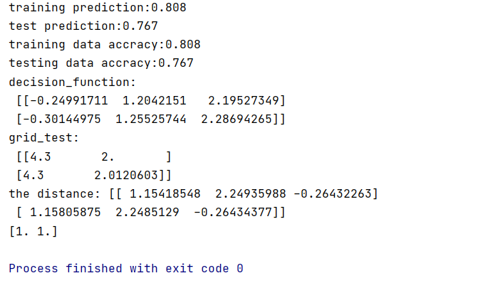
结果展示
可以看到分类效果和之前的k-means聚类效果图是差不多的。
有兴趣的可以看看k-means聚类进行分类:
使用k-means聚类对鸢尾花进行分类:https://www.cnblogs.com/hjk-airl/p/16410359.html
-
分类效果图

-
分类结果参数
总结
可以看到SVM鸢尾花分类和K-means聚类是不同的,但是都可以达到分类的效果。