卷积神经网络——vgg16网络及其python实现

1、介绍     

        VGG-16网络包括13个卷积层和3个全连接层，网络结构较LeNet-5等网络变得十分复杂，但同时也有不错的效果。VGG16有强大的拟合能力在当时取得了非常的效果，但同时VGG也有部分不足：
1、巨大参数量导致训练时间过长，调参难度较大；
2、模型所需内存容量大，VGG的权值文件很大，用到实际应用会比较困难。

2、结构原理 

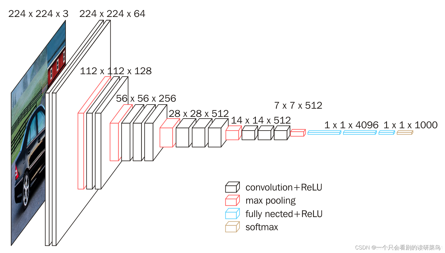
这是经典的vgg网络，输入图片大小为224*224。

下面这为官方给出的几种VGG结构图。

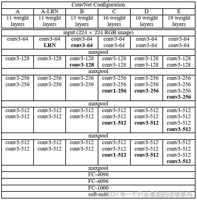
 现在多用的为D模型。

简单介绍下过程，输入224*224大小的图片，然后用两次64个3*3的卷积核进行全采集，也就是补零采集，保证特征不丢失，得到64*224*224的特征；池化层得到64*112*112；再利用128个3*3的卷积核进行特征采集两次，得到特征112*112*128；池化得到56*56*128大小特征.........反复这样操作，最后卷积完得到7*7*512的特征，然后利用全连接层进行展开，最后得到1000个特征，随后进行概率分类操作。

3、python实现

        选用的数据集为fashion数据集，具体请另外了解。数据可直接在库中导入，本文用class网络编写神经网络程序。

class VGG16(Model):
    def __init__(self):
        super(VGG16, self).__init__()
        self.c1 = Conv2D(filters=64, kernel_size=(3, 3), padding='same')  
        self.b1 = BatchNormalization()  
        self.a1 = Activation('relu')  
        self.c2 = Conv2D(filters=64, kernel_size=(3, 3), padding='same', )
        self.b2 = BatchNormalization() 
        self.a2 = Activation('relu')
        self.p1 = MaxPool2D(pool_size=(2, 2), strides=2, padding='same')
        self.d1 = Dropout(0.2) 
 
        self.c3 = Conv2D(filters=128, kernel_size=(3, 3), padding='same')
        self.b3 = BatchNormalization()  
        self.a3 = Activation('relu')  
        self.c4 = Conv2D(filters=128, kernel_size=(3, 3), padding='same')
        self.b4 = BatchNormalization()  
        self.a4 = Activation('relu')  
        self.p2 = MaxPool2D(pool_size=(2, 2), strides=2, padding='same')
        self.d2 = Dropout(0.2) 
 
        self.c5 = Conv2D(filters=256, kernel_size=(3, 3), padding='same')
        self.b5 = BatchNormalization()  
        self.a5 = Activation('relu')  
        self.c6 = Conv2D(filters=256, kernel_size=(3, 3), padding='same')
        self.b6 = BatchNormalization()  
        self.a6 = Activation('relu')  
        self.c7 = Conv2D(filters=256, kernel_size=(3, 3), padding='same')
        self.b7 = BatchNormalization()
        self.a7 = Activation('relu')
        self.p3 = MaxPool2D(pool_size=(2, 2), strides=2, padding='same')
        self.d3 = Dropout(0.2)
 
        self.c8 = Conv2D(filters=512, kernel_size=(3, 3), padding='same')
        self.b8 = BatchNormalization()
        self.a8 = Activation('relu')  
        self.c9 = Conv2D(filters=512, kernel_size=(3, 3), padding='same')
        self.b9 = BatchNormalization()  
        self.a9 = Activation('relu')  
        self.c10 = Conv2D(filters=512, kernel_size=(3, 3), padding='same')
        self.b10 = BatchNormalization()
        self.a10 = Activation('relu')
        self.p4 = MaxPool2D(pool_size=(2, 2), strides=2, padding='same')
        self.d4 = Dropout(0.2)
 
        self.c11 = Conv2D(filters=512, kernel_size=(3, 3), padding='same')
        self.b11 = BatchNormalization() 
        self.a11 = Activation('relu')  
        self.c12 = Conv2D(filters=512, kernel_size=(3, 3), padding='same')
        self.b12 = BatchNormalization()  
        self.a12 = Activation('relu')  
        self.c13 = Conv2D(filters=512, kernel_size=(3, 3), padding='same')
        self.b13 = BatchNormalization()
        self.a13 = Activation('relu')
        self.p5 = MaxPool2D(pool_size=(2, 2), strides=2, padding='same')
        self.d5 = Dropout(0.2)
 
        self.flatten = Flatten()
        self.f1 = Dense(512, activation='relu')
        self.d6 = Dropout(0.2)
        self.f2 = Dense(512, activation='relu')
        self.d7 = Dropout(0.2)
        self.f3 = Dense(10, activation='softmax')
 
    def call(self, x):
        x = self.c1(x)
        x = self.b1(x)
        x = self.a1(x)
        x = self.c2(x)
        x = self.b2(x)
        x = self.a2(x)
        x = self.p1(x)
        x = self.d1(x)
 
        x = self.c3(x)
        x = self.b3(x)
        x = self.a3(x)
        x = self.c4(x)
        x = self.b4(x)
        x = self.a4(x)
        x = self.p2(x)
        x = self.d2(x)
 
        x = self.c5(x)
        x = self.b5(x)
        x = self.a5(x)
        x = self.c6(x)
        x = self.b6(x)
        x = self.a6(x)
        x = self.c7(x)
        x = self.b7(x)
        x = self.a7(x)
        x = self.p3(x)
        x = self.d3(x)
 
        x = self.c8(x)
        x = self.b8(x)
        x = self.a8(x)
        x = self.c9(x)
        x = self.b9(x)
        x = self.a9(x)
        x = self.c10(x)
        x = self.b10(x)
        x = self.a10(x)
        x = self.p4(x)
        x = self.d4(x)
 
        x = self.c11(x)
        x = self.b11(x)
        x = self.a11(x)
        x = self.c12(x)
        x = self.b12(x)
        x = self.a12(x)
        x = self.c13(x)
        x = self.b13(x)
        x = self.a13(x)
        x = self.p5(x)
        x = self.d5(x)
 
        x = self.flatten(x)
        x = self.f1(x)
        x = self.d6(x)
        x = self.f2(x)
        x = self.d7(x)
        y = self.f3(x)
        return y
 
 
model = VGG16()

读取数据

import tensorflow as tf
import os
import numpy as np
from matplotlib import pyplot as plt
from tensorflow.keras.layers import Conv2D, BatchNormalization, Activation, MaxPool2D, Dropout, Flatten, Dense
from tensorflow.keras import Model
 
np.set_printoptions(threshold=np.inf)
 
fashion = tf.keras.datasets.fashion_mnist
(x_train, y_train), (x_test, y_test) = fashion.load_data()
x_train, x_test = x_train / 255.0, x_test / 255.0
x_train = x_train.reshape(x_train.shape[0], 28, 28, 1) 
x_test = x_test.reshape(x_test.shape[0], 28, 28, 1)

迭代训练

model.compile(optimizer='adam',
              loss=tf.keras.losses.SparseCategoricalCrossentropy(from_logits=False),
              metrics=['sparse_categorical_accuracy'])
cp_callback = tf.keras.callbacks.ModelCheckpoint(filepath=checkpoint_save_path,
                                                 save_weights_only=True,
                                                 save_best_only=True)
 
history = model.fit(x_train, y_train, batch_size=64, epochs=20, validation_data=(x_test, y_test), validation_freq=1,
                    callbacks=[cp_callback])

绘制结果图

acc = history.history['sparse_categorical_accuracy']
val_acc = history.history['val_sparse_categorical_accuracy']
loss = history.history['loss']
val_loss = history.history['val_loss']
 
plt.subplot(1, 2, 1)
plt.plot(acc, label='Training Accuracy')
plt.plot(val_acc, label='Validation Accuracy')
plt.title('Training and Validation Accuracy')
plt.legend()
 
plt.subplot(1, 2, 2)
plt.plot(loss, label='Training Loss')
plt.plot(val_loss, label='Validation Loss')
plt.title('Training and Validation Loss')
plt.legend()
plt.show()

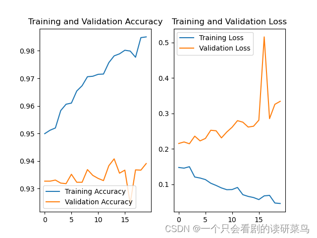
 虽然不是很稳定，但总的来说准确率还可以。