-
使用卷积神经网络实现猫狗分类任务
使用卷积神经网络在猫狗分类数据集上实现分类任务。
一、数据集下载链接
猫狗分类数据集链接 → 提取码:1uwy。
二、基础环境配置
- Windows10 + Anaconda3 + PyCharm 2019.3.3
- 安装CPU版本的TensorFlow
- 在PyCharm中配置好TensorFlow环境
三、训练及测试过程
-
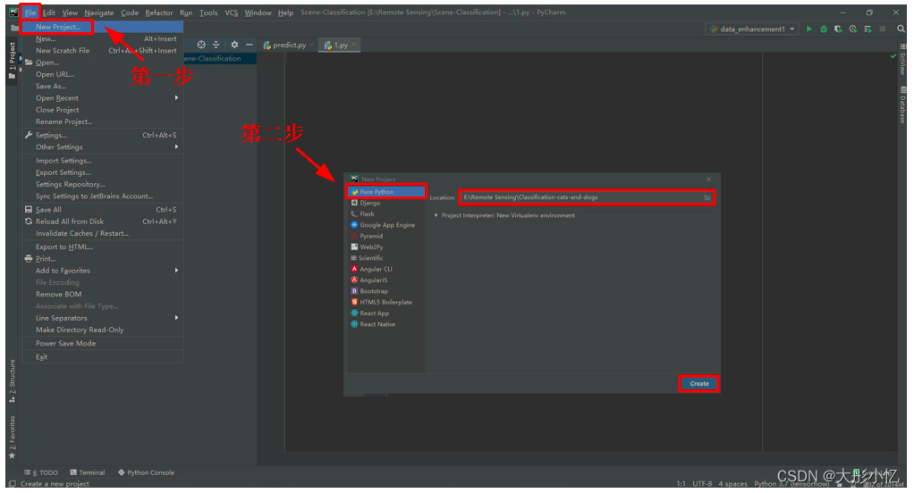
在PyCharm中新建猫狗分类项目
Classification-cats-and-dogs。第一步依次点击File→New Project...后,第二步点击Pure Python后选择好新建项目的位置,然后点击Create。
-
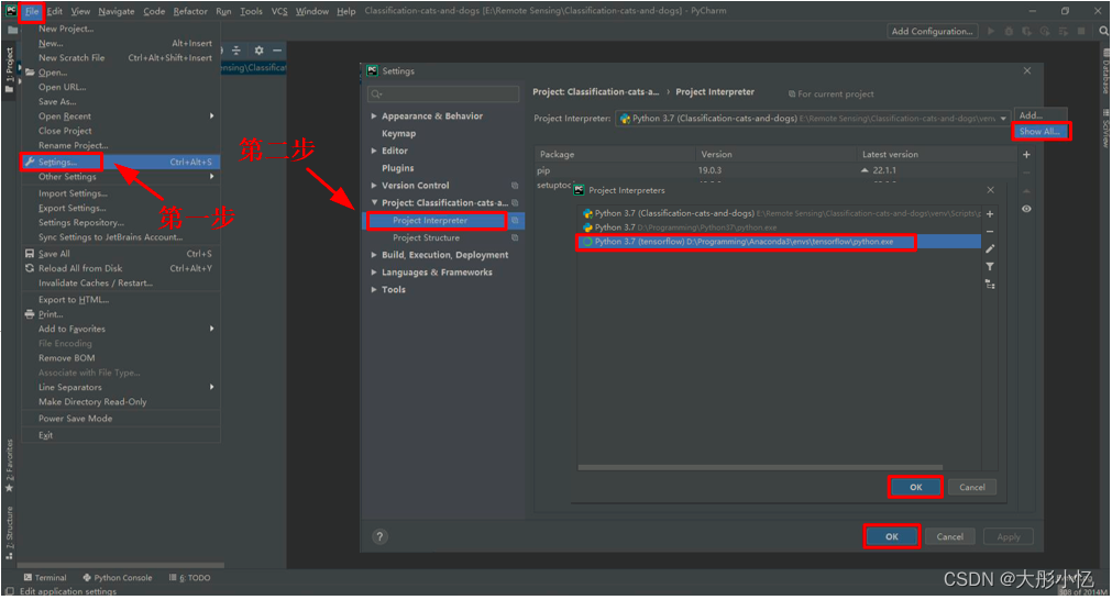
给新建的项目配置好TensorFlow环境。第一步依次点击
File→Settings...后,第二步点击Project Interpreter后,再点击Show All...选择tensorflow环境,然后再依次点击OK→OK。
-
在猫狗分类项目
Classification-cats-and-dogs中新建分类模型文件classification.py。第一步右击项目Classification-cats-and-dogs后依次选择New→Python File,第二步给新建的文件命名classification后回车。

-
classification.py文件的代码如下所示。
import os import tensorflow as tf from tensorflow.keras.optimizers import RMSprop from tensorflow.keras.preprocessing.image import ImageDataGenerator import matplotlib.pyplot as plt base_dir = 'E:/Remote Sensing/Data Set/cats_and_dogs' # 指定每一种数据的位置 train_dir = os.path.join(base_dir, 'train') validation_dir = os.path.join(base_dir, 'validation') # Directory with our training cat/dog pictures train_cats_dir = os.path.join(train_dir, 'cats') train_dogs_dir = os.path.join(train_dir, 'dogs') # Directory with our validation cat/dog pictures validation_cats_dir = os.path.join(validation_dir, 'cats') validation_dogs_dir = os.path.join(validation_dir, 'dogs') # 设计模型 model = tf.keras.models.Sequential([ # 我们的数据是150x150而且是三通道的,所以我们的输入应该设置为这样的格式。 tf.keras.layers.Conv2D(16, (3, 3), activation='relu', input_shape=(256, 256, 3)), tf.keras.layers.MaxPooling2D(2, 2), tf.keras.layers.Conv2D(32, (3, 3), activation='relu'), tf.keras.layers.MaxPooling2D(2, 2), tf.keras.layers.Conv2D(64, (3, 3), activation='relu'), tf.keras.layers.MaxPooling2D(2, 2), # Flatten the results to feed into a DNN tf.keras.layers.Flatten(), # 512 neuron hidden layer tf.keras.layers.Dense(512, activation='relu'), # 二分类只需要一个输出 tf.keras.layers.Dense(1, activation='sigmoid') ]) model.summary() # 打印模型相关信息 # 进行优化方法选择和一些超参数设置 # 因为只有两个分类。所以用2分类的交叉熵,使用RMSprop,学习率为0.001.优化指标为accuracy model.compile(optimizer=RMSprop(lr=0.001), loss='binary_crossentropy', metrics=['acc']) # 数据处理 # 把每个数据都放缩到0到1范围内 train_datagen = ImageDataGenerator(rescale=1.0 / 255.) test_datagen = ImageDataGenerator(rescale=1.0 / 255.) # 生成训练集的带标签的数据 train_generator = train_datagen.flow_from_directory(train_dir, # 训练图片的位置 batch_size=20, # 每一个投入多少张图片训练 class_mode='binary', # 设置我们需要的标签类型 target_size=(150, 150)) # 将图片统一大小 # 生成验证集带标签的数据 validation_generator = test_datagen.flow_from_directory(validation_dir, # 验证图片的位置 batch_size=20, # 每一个投入多少张图片训练 class_mode='binary', # 设置我们需要的标签类型 target_size=(150, 150)) # 将图片统一大小 # 进行训练 history = model.fit_generator(train_generator, validation_data=validation_generator, steps_per_epoch=100, epochs=15, validation_steps=50, verbose=2) # 保存训练的模型 model.save('model.h5') # 得到精度和损失值 acc = history.history['acc'] val_acc = history.history['val_acc'] loss = history.history['loss'] val_loss = history.history['val_loss'] epochs = range(len(acc)) # 得到迭代次数 # 绘制精度曲线 plt.plot(epochs, acc) plt.plot(epochs, val_acc) plt.title('Training and validation accuracy') plt.legend(('Training accuracy', 'validation accuracy')) plt.figure() # 绘制损失曲线 plt.plot(epochs, loss) plt.plot(epochs, val_loss) plt.legend(('Training loss', 'validation loss')) plt.title('Training and validation loss') plt.show()- 1
- 2
- 3
- 4
- 5
- 6
- 7
- 8
- 9
- 10
- 11
- 12
- 13
- 14
- 15
- 16
- 17
- 18
- 19
- 20
- 21
- 22
- 23
- 24
- 25
- 26
- 27
- 28
- 29
- 30
- 31
- 32
- 33
- 34
- 35
- 36
- 37
- 38
- 39
- 40
- 41
- 42
- 43
- 44
- 45
- 46
- 47
- 48
- 49
- 50
- 51
- 52
- 53
- 54
- 55
- 56
- 57
- 58
- 59
- 60
- 61
- 62
- 63
- 64
- 65
- 66
- 67
- 68
- 69
- 70
- 71
- 72
- 73
- 74
- 75
- 76
- 77
- 78
- 79
- 80
- 81
- 82
- 83
- 84
- 85
- 86
- 87
- 88
- 89
- 90
- 91
- 92
- 93
-
运行
classification.py文件,开始训练模型。
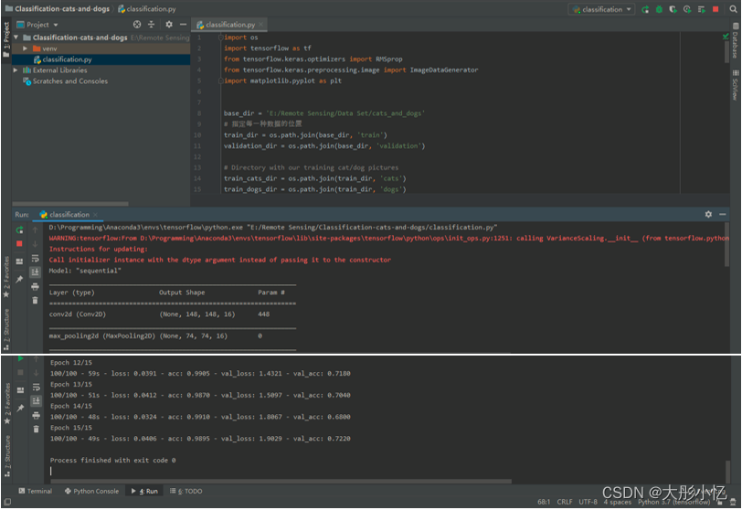
-
训练结束后可以在根路径下得到最终模型
model.h5,如下图所示。

还可以得到精度曲线和损失曲线,如下图所示。

分析曲线可以发现,存在着过拟合的现象,而且验证集的准确率比较低,下面将使用数据增强和dropout方式解决过拟合。 -
新建一个
classification_DataEnhancement and Dropout.py文件,在classification.py文件的基础上通过采用数据增强和dropout方式来对过拟合问题进行解决,代码如下所示。
import os import tensorflow as tf from tensorflow.keras.optimizers import RMSprop from tensorflow.keras.preprocessing.image import ImageDataGenerator import matplotlib.pyplot as plt base_dir = 'E:/Remote Sensing/Data Set/cats_and_dogs' train_dir = os.path.join(base_dir, 'train') validation_dir = os.path.join(base_dir, 'validation') train_cats_dir = os.path.join(train_dir, 'cats') train_dogs_dir = os.path.join(train_dir, 'dogs') validation_cats_dir = os.path.join(validation_dir, 'cats') validation_dogs_dir = os.path.join(validation_dir, 'dogs') # 模型处添加了dropout随机失效,也就是说有时候可能不用到某些神经元,失效率为0.5 model = tf.keras.models.Sequential([ tf.keras.layers.Conv2D(32, (3, 3), activation='relu', input_shape=(150, 150, 3)), tf.keras.layers.MaxPooling2D(2, 2), tf.keras.layers.Conv2D(64, (3, 3), activation='relu'), tf.keras.layers.MaxPooling2D(2, 2), tf.keras.layers.Conv2D(128, (3, 3), activation='relu'), tf.keras.layers.MaxPooling2D(2, 2), tf.keras.layers.Conv2D(128, (3, 3), activation='relu'), tf.keras.layers.MaxPooling2D(2, 2), tf.keras.layers.Dropout(0.5), tf.keras.layers.Flatten(), tf.keras.layers.Dense(512, activation='relu'), tf.keras.layers.Dense(1, activation='sigmoid') ]) model.compile(loss='binary_crossentropy', optimizer=RMSprop(lr=1e-4), metrics=['acc']) # 这里的代码进行了更新,原来这里只进行归一化处理,现在要进行数据增强。 train_datagen = ImageDataGenerator( rescale=1. / 255, rotation_range=40, width_shift_range=0.2, height_shift_range=0.2, shear_range=0.2, zoom_range=0.2, horizontal_flip=True, fill_mode='nearest') test_datagen = ImageDataGenerator(rescale=1. / 255) train_generator = train_datagen.flow_from_directory( train_dir, target_size=(150, 150), batch_size=20, class_mode='binary') validation_generator = test_datagen.flow_from_directory( validation_dir, target_size=(150, 150), batch_size=20, class_mode='binary') history = model.fit_generator( train_generator, steps_per_epoch=100, epochs=100, validation_data=validation_generator, validation_steps=50, verbose=2) # 保存训练的模型 model.save('model.h5') # 得到精度和损失值 acc = history.history['acc'] val_acc = history.history['val_acc'] loss = history.history['loss'] val_loss = history.history['val_loss'] epochs = range(len(acc)) # 得到迭代次数 # 绘制精度曲线 plt.plot(epochs, acc) plt.plot(epochs, val_acc) plt.title('Training and validation accuracy') plt.legend(('Training accuracy', 'validation accuracy')) plt.figure() # 绘制损失曲线 plt.plot(epochs, loss) plt.plot(epochs, val_loss) plt.legend(('Training loss', 'validation loss')) plt.title('Training and validation loss') plt.show()- 1
- 2
- 3
- 4
- 5
- 6
- 7
- 8
- 9
- 10
- 11
- 12
- 13
- 14
- 15
- 16
- 17
- 18
- 19
- 20
- 21
- 22
- 23
- 24
- 25
- 26
- 27
- 28
- 29
- 30
- 31
- 32
- 33
- 34
- 35
- 36
- 37
- 38
- 39
- 40
- 41
- 42
- 43
- 44
- 45
- 46
- 47
- 48
- 49
- 50
- 51
- 52
- 53
- 54
- 55
- 56
- 57
- 58
- 59
- 60
- 61
- 62
- 63
- 64
- 65
- 66
- 67
- 68
- 69
- 70
- 71
- 72
- 73
- 74
- 75
- 76
- 77
- 78
- 79
- 80
- 81
- 82
- 83
- 84
- 85
- 86
- 87
- 88
- 89
- 90
- 91
- 92
- 93
- 94
-
运行
classification_DataEnhancement and Dropout.py文件可以得到新的模型及精度和损失曲线如下图所示。

分析曲线可以发现,过拟合情况得到了改善。 -
新建一个
predict.py文件对需要测试的图片进行类别预测,代码如下所示。
# 预测 from tensorflow.keras.models import load_model import numpy as np from tensorflow.keras.preprocessing import image path = 'E:/Remote Sensing/Classification-cats-and-dogs/dog.jpeg' model = load_model('model.h5') img = image.load_img(path, target_size=(150, 150)) x = image.img_to_array(img) / 255.0 # 在第0维添加维度变为1x150x150x3,和我们模型的输入数据一样 x = np.expand_dims(x, axis=0) # np.vstack:按垂直方向(行顺序)堆叠数组构成一个新的数组,我们一次只有一个数据所以不这样也可以 images = np.vstack([x]) # batch_size批量大小,程序会分批次地预测测试数据,这样比每次预测一个样本会快 classes = model.predict(images, batch_size=1) if classes[0] > 0.5: print("It is a dog") else: print("It is a cat")- 1
- 2
- 3
- 4
- 5
- 6
- 7
- 8
- 9
- 10
- 11
- 12
- 13
- 14
- 15
- 16
- 17
- 18
- 19
- 20
- 在网上下载一张狗的图片,如下图所示。

运行predict.py文件,就可以得到分类结果,如下图所示。

在网上下载一张猫的图片,如下图所示。

运行predict.py文件,就可以得到分类结果,如下图所示。

- 新建
visual.py文件对每个卷积层的特征进行可视化,代码如下所示。
import numpy as np import matplotlib.pyplot as plt from tensorflow.keras.preprocessing.image import img_to_array, load_img import tensorflow as tf from tensorflow.keras.models import load_model np.seterr(divide='ignore', invalid='ignore') model = load_model('model.h5') # 让我们定义一个新模型,该模型将图像作为输入,并输出先前模型中所有层的中间表示。 successive_outputs = [layer.output for layer in model.layers[1:]] # 进行可视化模型搭建,设置输入和输出 visualization_model = tf.keras.models.Model(inputs=model.input, outputs=successive_outputs) # 选取一张随机的图片 img_path = 'E:/Remote Sensing/Classification-cats-and-dogs/dog.jpeg' img = load_img(img_path, target_size=(150, 150)) # 以指定大小读取图片 x = img_to_array(img) # 变成array x = x.reshape((1,) + x.shape) # 变成 (1, 150, 150, 3) # 统一范围到0到1 x /= 255 # 运行我们的模型,得到我们要画的图。 successive_feature_maps = visualization_model.predict(x) # 选取每一层的名字 layer_names = [layer.name for layer in model.layers] # 开始画图 for layer_name, feature_map in zip(layer_names, successive_feature_maps): if len(feature_map.shape) == 4: # 只绘制卷积层,池化层,不画全连接层。 n_features = feature_map.shape[-1] # 最后一维的大小,也就是通道数,也是我们提取的特征数 # feature_map的形状为 (1, size, size, n_features) size = feature_map.shape[1] # 我们将在此矩阵中平铺图像 display_grid = np.zeros((size, size * n_features)) for i in range(n_features): # 后期处理我们的特征,使其看起来更美观。 x = feature_map[0, :, :, i] x -= x.mean() x /= x.std() x *= 64 x += 128 x = np.clip(x, 0, 255).astype('uint8') # 我们把图片平铺到这个大矩阵中 display_grid[:, i * size: (i + 1) * size] = x # 绘制这个矩阵 scale = 20. / n_features plt.figure(figsize=(scale * n_features, scale)) # 设置图片大小 plt.title(layer_name) # 设置题目 plt.grid(False) # 不绘制网格线 # aspect='auto'自动控制轴的长宽比。 这方面对于图像特别相关,因为它可能会扭曲图像,即像素不会是正方形的。 # cmap='viridis'设置图像的颜色变化 plt.imshow(display_grid, aspect='auto', cmap='viridis') plt.show()- 1
- 2
- 3
- 4
- 5
- 6
- 7
- 8
- 9
- 10
- 11
- 12
- 13
- 14
- 15
- 16
- 17
- 18
- 19
- 20
- 21
- 22
- 23
- 24
- 25
- 26
- 27
- 28
- 29
- 30
- 31
- 32
- 33
- 34
- 35
- 36
- 37
- 38
- 39
- 40
- 41
- 42
- 43
- 44
- 45
- 46
- 47
- 48
- 49
- 50
- 51
- 52
- 53
- 54
- 55
- 56
- 57
- 运行可视化代码后得到的结果如下图所示。

分析可视化结果可以发现,越浅的层对应的特征图中包含的图像底层像素信息越多,轮廓越清晰,与原图更为相近;随着层数的增加,所得到的特征图中包含的有效特征越来越少,特征图变得越来越抽象,稀疏程度也更高。
参考文章:https://blog.csdn.net/weixin_43398590/article/details/105173936
https://blog.csdn.net/weixin_43398590/article/details/105174367?spm=1001.2014.3001.5502 -
相关阅读:
【小程序项目开发-- 京东商城】uni-app之自定义搜索组件(下) -- 搜索历史
【推荐系统】:协同过滤和基于内容过滤概述
LeetCode 0168. Excel表列名称
Unity发布的手机游戏插上耳机也是外音
【Git】如何在Vscode中使用码云(Gitee)实现远程代码仓库与本地同步?(新手图文教程)
Avalonia项目打包安装包
简单工厂和工厂方法模式
02_Alibaba微服务组件Nacos注册中心
discuzx3.4帖子表pre_forum_post中invisible字段说明
【C语言】const 关键字
- 原文地址:https://blog.csdn.net/HUAI_BI_TONG/article/details/124746643