视觉SLAM十四讲笔记-8-1

文章目录

视觉SLAM十四讲笔记-8-1
视觉里程计2

视觉里程计2

主要目标：
1.理解光流法跟踪特征点的原理；
2.理解直接法是如何估计相机位姿的；
3.实现多层直接法的计算。
直接法是视觉里程计中的另一个分支，它与特征点有很大不同。虽然它还没有成为视觉里程计的主流，但经过近几年的发展，直接法在一定程度上已经能和特征点法平分秋色。

8.1 直接法的引出

上一章中介绍了特征点法估计相机运动的方法。特征点法至少存在以下缺点：
1.关键点的提取与描述子的计算非常耗时；
2.使用特征点时，忽略了除特征点以外的所有信息。只使用特征点丢弃了大部分可能有用的图像信息；
3.相机有时会运动到特征丢失的地方，这些地方往往没有明显的纹理信息。这时可能找不到足够的匹配点来计算相机运动。
为了克服这些缺点，有以下几种思路：
1.保留特征点，但只计算关键点，不计算描述子。 同时，使用光流法(Optical Flow) 跟踪特征点的运动。这样可以回避计算和匹配描述子带来的时间。光流本身的计算时间要小于描述子的计算和匹配。(这种方法仍然使用特征点，只是把匹配描述子替换成了光流跟踪，估计相机运动仍然使用对极几何、PnP 和 ICP算法。这依然会要求提取到的关键点具有可区别性)
2.只计算关键点，不计算描述子。　同时，使用直接法(Direct Method) 计算特征点在下一时刻图像中的位置。这同样可以跳过描述子的计算过程，也省去了光流的计算时间。(这种方法会根据图像的像素灰度信息同时估计相机运动和点的投影，不要求提取到的点必须是角点，甚至可以是随机的选点)
使用特征点法估计相机运动时，把特征点看作固定在三维空间的不动点。根据它们在相机中的投影位置，通过最小化重投影误差优化相机运动。在这个过程中需要精确地知道空间点在两个相机中投影后的像素位置。在直接法中，并不需要知道点与点之间的对应关系，而是通过最小化光度误差(Photometric error) 来求得它们。
直接法根据像素的亮度信息估计相机的运动，可以完全不用计算关键点和描述子，于是，既可以避免了特征的计算时间，也避免了特征缺失的情况。只要场景中存在明暗变化(可以是渐变，不形成局部的图像梯度)，直接法就能工作。
根据像素的数量，直接法分为稀疏、稠密和半稠密三种。与特征点法只能重构稀疏特征点(稀疏地图)相比，直接法还具有恢复半稠密地图或者稠密结构的能力。

8.2 2D光流

直接法是从光流演变而来的。它们非常相似，具有相同的假设条件。光流描述了像素在图像中的运动，而直接法则附带着一个相机运动模型。为了说明直接法，先来介绍光流。
光流是一种描述像素随时间在图像之间运动的方法。
图片链接：link
在这里插入图片描述
如上图所示，随着时间的流逝，同一个像素会在图像中运动，希望跟踪它的运动过程。其中，计算部分像素的运动称为稀疏光流，计算所有像素的称为稠密光流。稀疏光流以 Lucas-Kanade 光流为代表，并可以在 SLAM 中用于跟踪特征点位置。稠密光流以 Horn-Schunck 光流为代表。因此，本节主要介绍 Lucas-Kanade 光流，也称为 LK 光流。

8.2.1 Lucas-Kanade光流

在 LK 光流中，认为来自相机的图像是随时间变化的。图像可以看做时间的函数: $I (t)$ 。那么，一个在 $t$ 时刻，位于 $(x, y)$ 处的像素，它的灰度可以写成：
$I (x, y, t)$
这种方式把图像看成了关于位置与时间的函数，它的值域就是图像中像素的灰度。现在考虑某个固定的空间点，它在 $t$ 时刻的像素坐标为 $x, y$ 。由于相机的运动，它的图像坐标将发生变化。希望估计这个空间点在其他时刻图像中的位置。怎么估计尼?这里要引入光流法的基本假设。
灰度不变假设：同一个空间点的像素灰度值，在各个图像中是固定不变的。
对于 $t$ 时刻位于 $(x, y)$ 处的像素，设 $t + d t$ 时刻它运动到 $(x + d x, y + d y)$ 处。由于灰度不变，有：
$I (x + d x, y + d y, t + d t) = I (x, y, t)$
注意灰度不变假设是一个很强的假设，实际上很可能不成立。事实上，由于物体的材质不同，像素会出现高光和阴影部分；有时，相机会自动调整曝光参数，使得图像整体变亮或者变暗。这时灰度不变假设都是不成立的，因此光流的结果也不一定可靠。暂时认为该假设成立，看看如何计算像素的运动。
对左边进行泰勒展开，保留一阶项，得：
$\approx I(x,y,t) + \frac{\partial I}{\partial x} dx + \frac{\partial I}{\partial y}dy + \frac{\partial I}{\partial t}dt$
因为假设了灰度不变，于是下一个时刻的灰度等于之前的灰度，从而：
$\frac{\partial I}{\partial x} dx + \frac{\partial I}{\partial y}dy + \frac{\partial I}{\partial t}dt = 0$
两边除以 $d t$ ，得：
$\frac{\partial I}{\partial x} \frac{dx}{dt} + \frac{\partial I}{\partial y}\frac{dy}{dt} = -\frac{\partial I}{\partial t}$
其实 $\frac{dx}{dt}$ 为像素在 $x$ 轴上的运动速度，而 $\frac{dy}{dt}$ 为像素在 $y$ 轴上的运动速度，把它们记作 $u, v$ 。

同时， $\frac{\partial I}{\partial x}$ 为图像在该点处 $x$ 方向的梯度， $\frac{\partial I}{\partial y}$ 为图像在该点处 $y$ 方向的梯度，记为 $I_x,I_y$ 。把图像灰度对时间的变化量记为 $I_t$ ，写成矩阵的形式：

[\begin{matrix} I_{x} & I_{y} \end{matrix}]

[\begin{matrix} u \\ v \end{matrix}]

= -I_t

[I_{x} I_{y}] [u v] = - I_{t}

想计算的是像素的运动

u, v

，但是该式是带有两个变量的一次方程，仅凭它无法计算出

u, v

。因此，必须引入额外的约束来计算

u, v

。
在 LK 光流中，假设某一个窗口内的像素具有相同的运动。考虑一个大小为

w * w

的窗口，它含有

w^2

数量的像素。该窗口内像素具有同样的运动，因此共有

w^2

个方程：

[\begin{matrix} I_{x} & I_{y} \end{matrix}]

记：

\begin{matrix} {[I_{x}, I_{y}]}_{1} \\ ⋮ \\ {[I_{x}, I_{y}]}_{k} \end{matrix}

于是整个方程为：

[\begin{matrix} u \\ v \end{matrix}]

这是一个关于

u, v

的超定线性方程，传统解法是求最小二乘解。最小二乘经常被用到：

\begin{array}{l} u \\ v \end{array}

这样就得到了像素在图像间的运动速度

u, v

。当

t

取离散时刻而不是连续时间时，可以估计某块像素在若干个图像中出现的位置。
由于像素梯度仅在局部有效，所以如果一次迭代不够好，可以迭代几次这个方程。在 SLAM 中，LK 光流经常被用来跟踪角点的运动。

8.3 实践：LK光流

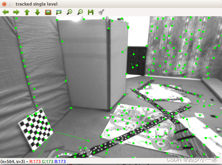
8.3.1 使用 LK 光流

在本节中，用 OpenCV 的光流来追踪上面的特征点。同时也手动实现一个 LK 光流。
使用两张来自 Euroc 数据集的示例图像，在第一张图像中提取角点，然后用光流法追踪它们在第二张图像中的位置。
OpenCV 的光流在使用上十分简单，只需调用 cv::calcOpticalFlowPyrLK 函数，提供前后两张图像及对应的特征点，即可得到追踪后的点，以及各点的状态、误差。可以根据 status 变量是否为 1 来确定对应的点是否被正确追踪到。

mkdir optical_flow
cd optical_flow/
code .
1
2
3

//launch.json
{
    // Use IntelliSense to learn about possible attributes.
    // Hover to view descriptions of existing attributes.
    // For more information, visit: https://go.microsoft.com/fwlink/?linkid=830387
    "version": "0.2.0",
    "configurations": [
        {
            "name": "g++ - 生成和调试活动文件",
            "type": "cppdbg",
            "request":"launch",
            "program":"${workspaceFolder}/build/optical_flow",
            "args": [],
            "stopAtEntry": false,
            "cwd": "${workspaceFolder}",
            "environment": [],
            "externalConsole": false,
            "MIMode": "gdb",
            "setupCommands": [
                {
                    "description": "为 gdb 启动整齐打印",
                    "text": "-enable-pretty-printing",
                    "ignoreFailures": true
                }
            ],
            "preLaunchTask": "Build",
            "miDebuggerPath": "/usr/bin/gdb"
        }
    ]
}
1
2
3
4
5
6
7
8
9
10
11
12
13
14
15
16
17
18
19
20
21
22
23
24
25
26
27
28
29
30

//tasks.json
{
	"version": "2.0.0",
	"options":{
		"cwd": "${workspaceFolder}/build"   //指明在哪个文件夹下做下面这些指令
	},
	"tasks": [
		{
			"type": "shell",
			"label": "cmake",   //label就是这个task的名字,这个task的名字叫cmake
			"command": "cmake", //command就是要执行什么命令,这个task要执行的任务是cmake
			"args":[
				".."
			]
		},
		{
			"label": "make",  //这个task的名字叫make
			"group": {
				"kind": "build",
				"isDefault": true
			},
			"command": "make",  //这个task要执行的任务是make
			"args": [

			]
		},
		{
			"label": "Build",
			"dependsOrder": "sequence", //按列出的顺序执行任务依赖项
			"dependsOn":[				//这个label依赖于上面两个label
				"cmake",
				"make"
			]
		}
	]
}
1
2
3
4
5
6
7
8
9
10
11
12
13
14
15
16
17
18
19
20
21
22
23
24
25
26
27
28
29
30
31
32
33
34
35
36

#CMakeLists.txt
cmake_minimum_required(VERSION 3.0)

project(OPTICALFLOW)

#在g++编译时，添加编译参数，比如-Wall可以输出一些警告信息
set(CMAKE_CXX_FLAGS "${CMAKE_CXX_FLAGS} -Wall -std=c++14")

#一定要加上这句话，加上这个生成的可执行文件才是可以Debug的，不然不加或者是Release的话生成的可执行文件是无法进行调试的
set(CMAKE_BUILD_TYPE Debug)

list( APPEND CMAKE_MODULE_PATH /home/lss/Downloads/g2o/cmake_modules )
set(G2O_ROOT /usr/local/include/g2o)

# 为使用 sophus，需要使用find_package命令找到它
find_package(Sophus REQUIRED)
include_directories( ${Sophus_INCLUDE_DIRS} )

# Eigen
include_directories("/usr/include/eigen3")

find_package(Pangolin REQUIRED)
include_directories(${Pangolin_INCLUDE_DIRS})

find_package (glog 0.6.0 REQUIRED)


#此工程要调用opencv库，因此需要添加opancv头文件和链接库
#寻找OpenCV库
find_package(OpenCV REQUIRED)
#添加头文件
include_directories(${OpenCV_INCLUDE_DIRS})

# g2o
find_package(G2O REQUIRED)
include_directories(${G2O_INCLUDE_DIRS})

add_executable(optical_flow optical_flow.cpp)

#链接OpenCV库,Ceres库，
target_link_libraries(optical_flow ${OpenCV_LIBS} ${G2O_CORE_LIBRARY} ${G2O_STUFF_LIBRARY} glog::glog)
target_link_libraries(optical_flow Sophus::Sophus)
target_link_libraries(optical_flow ${Pangolin_LIBRARIES})
1
2
3
4
5
6
7
8
9
10
11
12
13
14
15
16
17
18
19
20
21
22
23
24
25
26
27
28
29
30
31
32
33
34
35
36
37
38
39
40
41
42
43

#include <opencv2/opencv.hpp>
#include <string>
#include <chrono>
#include <Eigen/Core>
#include <Eigen/Dense>
#include <algorithm>
#include <chrono>

using namespace std;
using namespace cv;

string file_1 = "./LK1.png";  // first image
string file_2 = "./LK2.png";  // second image

int main(int argc, char **argv)
{
    //---读取图像
    Mat img1 = imread(file_1, 0);
    Mat img2 = imread(file_2, 0);
    assert(img1.data && img2.data && "Can not load images!");

    //key points, using GFTT here
    vector<KeyPoint> kp1;
    Ptr<GFTTDetector> detector = GFTTDetector::create(500, 0.01, 20); //maximum 500 keypoints
    detector->detect(img1, kp1);

    //using opebcv's flow for validation
    vector<Point2f> pt1, pt2;
    for(auto &kp : kp1) pt1.push_back(kp.pt);
    vector<uchar> status;
    vector<float> error;

    chrono::steady_clock::time_point t1 = chrono::steady_clock::now();
    cv::calcOpticalFlowPyrLK(img1, img2, pt1, pt2, status, error);
    chrono::steady_clock::time_point t2 = chrono::steady_clock::now();
    auto time_used = chrono::duration_cast<chrono::duration<double>>(t2 - t1);
    cout << "optical flow by opencv: " << time_used.count() << endl;
	

	Mat img2_CV;
    cv::cvtColor(img2, img2_CV, CV_GRAY2BGR);
    for (int i = 0; i < pt2.size(); i++) {
        // 根据LK光流函数输出得到的状态变量status来确定对应点是否被正确跟踪o到
        if (status[i]) {
            // 绘制跟踪到的点为圆点
            cv::circle(img2_CV, pt2[i], 2, cv::Scalar(0, 250, 0), 2);
            // 跟踪点的运动方向
            cv::line(img2_CV, pt1[i], pt2[i], cv::Scalar(0, 250, 0));
        }
    }

    cv::imshow("tracked by opencv", img2_CV);
    cv::waitKey(0);
    
    return 0;
}
1
2
3
4
5
6
7
8
9
10
11
12
13
14
15
16
17
18
19
20
21
22
23
24
25
26
27
28
29
30
31
32
33
34
35
36
37
38
39
40
41
42
43
44
45
46
47
48
49
50
51
52
53
54
55
56

请添加图片描述
上面程序中首先用 OpenCV 的光流追踪上面的 GFTT 角点，然后用光流追踪它们在第二张图像中的位置。

8.3.2 用高斯牛顿法实现光流

单层光流：光流可以看成是一个优化问题：通过最小化灰度误差估计最优的像素偏移。
下面实现一个基于高斯牛顿法的光流。
在 OpticalFlowSingleLevel 函数中实现了单层光流函数，其中调用了 cv::paraller_for_ 并行调用 OpticalFlowTracker::calculateOpticalFlow，该函数计算指定范围内特征点的光流。这个并行 for 循环内部是 Intel tbb 库实现的，只需按照其接口，将函数本体定义出来，然后将函数作为 std::function 对象传递给它。

#include <opencv2/opencv.hpp>
#include <string>
#include <chrono>
#include <Eigen/Core>
#include <Eigen/Dense>
#include <algorithm>
#include <chrono>

using namespace std;
using namespace cv;

string file_1 = "./LK1.png"; // first image
string file_2 = "./LK2.png"; // second image

// OPtical flow tracker and interface
//光流跟踪器类
class OpticalFlowTracker
{
public:
    OpticalFlowTracker(
        const Mat &img1_,
        const Mat &img2_,
        const vector<KeyPoint> &kp1_,
        vector<KeyPoint> &kp2_,
        vector<bool> &success_,
        bool inverse_ = true, bool has_initial_ = false) : img1(img1_), img2(img2_), kp1(kp1_), kp2(kp2_), success(success_), inverse(inverse_), has_initial(has_initial_) {}
    //计算指定range范围内的特征点的光流
    void calculateOpticalFlow(const Range &range);

private:
    const Mat &img1;
    const Mat &img2;
    const vector<KeyPoint> &kp1;
    vector<KeyPoint> &kp2;
    vector<bool> &success;
    bool inverse = true;
    bool has_initial = false;
};

/**
 * single level optical flow
 * @param [in] img1 the first image
 * @param [in] img2 the second image
 * @param [in] kp1 keypoints in img1
 * @param [in|out] kp2 keypoints in img2, if empty, use initial guess in kp1
 * @param [out] success true if a keypoint is tracked successfully
 * @param [in] inverse use inverse formulation?
 */
//单层光流
void OpticalFlowSingleLevel(
    const Mat &img1,
    const Mat &img2,
    const vector<KeyPoint> &kp1,
    vector<KeyPoint> &kp2,
    vector<bool> &success,
    bool inverse = false, bool has_initial = false);

/**
 * get a gray scale value from reference image (bi-linear interpolated)
 * @param img
 * @param x
 * @param y
 * @return the interpolated value of this pixel
 */
//使用双线性内插法来估计一个点的像素：
//f(x,y) \approx f(0,0)(1-x)(1-y) + f(1,0)x(1-y)+f(0,1)(1-x)y + f(1,1)xy
inline float GetPixelValue(const cv::Mat &img, float x, float y)
{
    // boundary check
    if (x < 0)
        x = 0;
    if (y < 0)
        y = 0;
    if (x >= img.cols - 1)
        x = img.cols - 2;
    if (y >= img.rows - 1)
        y = img.rows - 2;

    float xx = x - floor(x);
    float yy = y - floor(y);
    int x_a1 = std::min(img.cols - 1, int(x) + 1);
    int y_a1 = std::min(img.rows - 1, int(y) + 1);

    return (1 - xx) * (1 - yy) * img.at<uchar>(y, x) + xx * (1 - yy) * img.at<uchar>(y, x_a1) + (1 - xx) * yy * img.at<uchar>(y_a1, x) + xx * yy * img.at<uchar>(y_a1, x_a1);
}

int main(int argc, char **argv)
{
    //---读取图像
    Mat img1 = imread(file_1, 0);
    Mat img2 = imread(file_2, 0);
    assert(img1.data && img2.data && "Can not load images!");

    // key points, using GFTT here
    vector<KeyPoint> kp1;
    Ptr<GFTTDetector> detector = GFTTDetector::create(500, 0.01, 20); // maximum 500 keypoints
    detector->detect(img1, kp1);

    //now lets track these key points in the second image
    //first use single level LK in the validation picture
    vector<KeyPoint> kp2_single;
    vector<bool> success_single;
    OpticalFlowSingleLevel(img1, img2, kp1, kp2_single, success_single);

    Mat img2_single;
    cv::cvtColor(img2, img2_single, CV_GRAY2BGR);
    for (int i = 0; i < kp2_single.size(); i++) {
        if (success_single[i]) {
            cv::circle(img2_single, kp2_single[i].pt, 2, cv::Scalar(0, 250, 0), 2);
            cv::line(img2_single, kp1[i].pt, kp2_single[i].pt, cv::Scalar(0, 250, 0));
        }
    }
    cv::imshow("tracked single level", img2_single);


    // using opencv's flow for validation
    vector<Point2f> pt1, pt2;
    for (auto &kp : kp1)
        pt1.push_back(kp.pt);
    vector<uchar> status;
    vector<float> error;
    chrono::steady_clock::time_point t1 = chrono::steady_clock::now();
    cv::calcOpticalFlowPyrLK(img1, img2, pt1, pt2, status, error);
    chrono::steady_clock::time_point t2 = chrono::steady_clock::now();
    auto time_used = chrono::duration_cast<chrono::duration<double>>(t2 - t1);
    cout << "optical flow by opencv: " << time_used.count() << endl;

    Mat img2_CV;
    cv::cvtColor(img2, img2_CV, CV_GRAY2BGR);
    for (int i = 0; i < pt2.size(); i++) {
        // 根据LK光流函数输出得到的状态变量status来确定对应点是否被正确跟踪o到
        if (status[i]) {
            // 绘制跟踪到的点为圆点
            cv::circle(img2_CV, pt2[i], 2, cv::Scalar(0, 250, 0), 2);
            // 跟踪点的运动方向
            cv::line(img2_CV, pt1[i], pt2[i], cv::Scalar(0, 250, 0));
        }
    }

    cv::imshow("tracked by opencv", img2_CV);
    cv::waitKey(0);


    return 0;
}

//单层光流
void OpticalFlowSingleLevel(
    const Mat &img1,
    const Mat &img2,
    const vector<KeyPoint> &kp1,
    vector<KeyPoint> &kp2,
    vector<bool> &success,
    bool inverse, bool has_initial)
{
    kp2.resize(kp1.size());
    success.resize(kp1.size());
    OpticalFlowTracker tracker(img1, img2, kp1, kp2, success, inverse, has_initial);
    parallel_for_(Range(0, kp1.size()), std::bind(&OpticalFlowTracker::calculateOpticalFlow, &tracker, placeholders::_1));
}

//计算指定range范围内的特征点的光流
void OpticalFlowTracker::calculateOpticalFlow(const Range &range)
{
    // parameters
    int half_patch_size = 4; //窗口的大小为 8 * 8
    int iterations = 10; //每一个角点迭代 10 次
    //总共循环的次数为 kp1.size()
    for (size_t i = range.start; i < range.end; ++i)
    {
        auto kp = kp1[i];
        double dx = 0, dy = 0; // dx, dy need to be estimated
        if (has_initial)
        {
            dx = kp2[i].pt.x - kp.pt.x;
            dy = kp2[i].pt.y - kp.pt.y;
        }
        double cost = 0, lastcost = 0;
        bool succ = true; // indicate if this point succeeded

        // Gauss-Newton iterations
        Eigen::Matrix2d H = Eigen::Matrix2d::Zero(); // hessian
        Eigen::Vector2d b = Eigen::Vector2d::Zero(); // bias
        Eigen::Vector2d J;                           // jacobian
        for (int iter = 0; iter < iterations; ++iter)
        {
            if (inverse == false)
            {
                H = Eigen::Matrix2d::Zero();
                b = Eigen::Vector2d::Zero();
            }
            else
            {
                // only reset b
                b = Eigen::Vector2d::Zero();
            }

            cost = 0;
            // compute cost and jacobian
            for (int x = -half_patch_size; x < half_patch_size; ++x)
            {
                for (int y = -half_patch_size; y < half_patch_size; ++y)
                {
                    //计算误差
                    double error = GetPixelValue(img1, kp.pt.x + x, kp.pt.y + y) -
                                   GetPixelValue(img2, kp.pt.x + x + dx, kp.pt.y + y + dy);;

                    if (inverse == false)   //雅可比矩阵，为第二个图像在x+dx,y+dy处的梯度。梯度上面已讲
                    {
                        J = -1.0 * Eigen::Vector2d(
                                       0.5 * (GetPixelValue(img2, kp.pt.x + dx + x + 1, kp.pt.y + dy + y) -
                                              GetPixelValue(img2, kp.pt.x + dx + x - 1, kp.pt.y + dy + y)),
                                       0.5 * (GetPixelValue(img2, kp.pt.x + dx + x, kp.pt.y + dy + y + 1) -
                                              GetPixelValue(img2, kp.pt.x + dx + x, kp.pt.y + dy + y - 1)));
                    }
                    else if (iter == 0) //反向光流，计算第一张图像的雅可比矩阵，10次迭代只计算一次
                    {
                        // in inverse mode, J keeps same for all iterations
                        // NOTE this J does not change when dx, dy is updated, so we can store it and only compute error
                        J = -1.0 * Eigen::Vector2d(
                                       0.5 * (GetPixelValue(img1, kp.pt.x + x + 1, kp.pt.y + y) -
                                              GetPixelValue(img1, kp.pt.x + x - 1, kp.pt.y + y)),
                                       0.5 * (GetPixelValue(img1, kp.pt.x + x, kp.pt.y + y + 1) -
                                              GetPixelValue(img1, kp.pt.x + x, kp.pt.y + y - 1)));
                    }
                    // compute H,b and set cost
                    b += -error * J;
                    cost += error * error;
                    if (inverse == false || iter == 0)
                    {
                        // also update H
                        H += J * J.transpose();
                    }
                }
            }

            // compute update
            Eigen::Vector2d update = H.ldlt().solve(b);

            if (std::isnan(update[0]))
            {
                // sometimes occurred when we have a black or white patch and H is irreversible
                cout << "update is nan" << endl;
                succ = false;
                break;
            }

            // update dx, dy
            dx += update[0];
            dy += update[1];
            lastcost = cost;
            succ = true;

            if (update.norm() < 1e-2)
            {
                // converge
                break;
            }
        }

        success[i] = succ;
        // set kp2
        kp2[i].pt = kp.pt + Point2f(dx, dy);
    }
}
1
2
3
4
5
6
7
8
9
10
11
12
13
14
15
16
17
18
19
20
21
22
23
24
25
26
27
28
29
30
31
32
33
34
35
36
37
38
39
40
41
42
43
44
45
46
47
48
49
50
51
52
53
54
55
56
57
58
59
60
61
62
63
64
65
66
67
68
69
70
71
72
73
74
75
76
77
78
79
80
81
82
83
84
85
86
87
88
89
90
91
92
93
94
95
96
97
98
99
100
101
102
103
104
105
106
107
108
109
110
111
112
113
114
115
116
117
118
119
120
121
122
123
124
125
126
127
128
129
130
131
132
133
134
135
136
137
138
139
140
141
142
143
144
145
146
147
148
149
150
151
152
153
154
155
156
157
158
159
160
161
162
163
164
165
166
167
168
169
170
171
172
173
174
175
176
177
178
179
180
181
182
183
184
185
186
187
188
189
190
191
192
193
194
195
196
197
198
199
200
201
202
203
204
205
206
207
208
209
210
211
212
213
214
215
216
217
218
219
220
221
222
223
224
225
226
227
228
229
230
231
232
233
234
235
236
237
238
239
240
241
242
243
244
245
246
247
248
249
250
251
252
253
254
255
256
257
258
259
260
261
262
263
264
265

运行结果：
请添加图片描述
在具体函数实现中，求解这样一个问题：
$\min _{\Delta x, \Delta y}\left\|\mathbf{I}_{1}(x, y)-\mathbf{I}_{2}(x+\Delta x, y+\Delta y)\right\|_{2}^{2}$
因此，残差为括号内部的部分，对应的雅克比为第二个图像在 $x+\Delta x，y+\Delta y$ 处的梯度。此外，这里的梯度也可以用第一个图像中的梯度 $I_1(x,y)$ 来代替。这种代替方法称为反向光流法。在反向光流法中， $I_1(x,y)$ 的梯度是保持不变的，可以在第一次迭代时保留计算的结果。在后续迭代中使用。当雅克比不变时， $H$ 矩阵不变，每次迭代只需要计算残差。

8.3.3 多层光流

把光流写成优化问题，就必须假设优化的初始值靠近最优值，才能在一定程度上保障算法的收敛。如果相机运行较快，两张图像差异明显，那么单层图像光流法容易达到一个局部极小值。这种情况可以引入图像金字塔来改善。
图像金字塔是指对同一个图像进行缩放，得到不同分辨率下的图像。以原始图像作为金字塔底层，每往上一层，就对下层图像进行一定倍率的缩放，就得到了一个图像金字塔。然后，在计算光流时，先从顶层的图像开始计算，然后把上一层的追踪结果作为下一层光流的初始值。由于上层的图像相对粗糙，所以这个过程也称为由粗到精的光流。
图像金字塔和光流由粗到精的过程如下图所示，图片来源：link
在这里插入图片描述
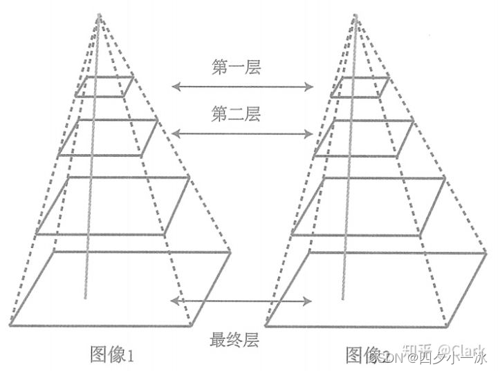
由粗到精的好处在于，当原始图像的像素运动较大时，在金字塔顶层的图像来看，运动仍然在一个小的范围内。
在上述代码中添加多层光流的代码：

#include <opencv2/opencv.hpp>
#include <string>
#include <chrono>
#include <Eigen/Core>
#include <Eigen/Dense>
#include <algorithm>
#include <chrono>

using namespace std;
using namespace cv;

string file_1 = "./LK1.png"; // first image
string file_2 = "./LK2.png"; // second image

// OPtical flow tracker and interface
//光流跟踪器类
class OpticalFlowTracker
{
public:
    OpticalFlowTracker(
        const Mat &img1_,
        const Mat &img2_,
        const vector<KeyPoint> &kp1_,
        vector<KeyPoint> &kp2_,
        vector<bool> &success_,
        bool inverse_ = true, bool has_initial_ = false) : img1(img1_), img2(img2_), kp1(kp1_), kp2(kp2_), success(success_), inverse(inverse_), has_initial(has_initial_) {}
    //计算指定range范围内的特征点的光流
    void calculateOpticalFlow(const Range &range);

private:
    const Mat &img1;
    const Mat &img2;
    const vector<KeyPoint> &kp1;
    vector<KeyPoint> &kp2;
    vector<bool> &success;
    bool inverse = true;
    bool has_initial = false;
};

/**
 * single level optical flow
 * @param [in] img1 the first image
 * @param [in] img2 the second image
 * @param [in] kp1 keypoints in img1
 * @param [in|out] kp2 keypoints in img2, if empty, use initial guess in kp1
 * @param [out] success true if a keypoint is tracked successfully
 * @param [in] inverse use inverse formulation?
 */
//单层光流
void OpticalFlowSingleLevel(
    const Mat &img1,
    const Mat &img2,
    const vector<KeyPoint> &kp1,
    vector<KeyPoint> &kp2,
    vector<bool> &success,
    bool inverse = false, bool has_initial = false);

/**
 * multi level optical flow, scale of pyramid is set to 2 by default
 * the image pyramid will be create inside the function
 * @param [in] img1 the first pyramid
 * @param [in] img2 the second pyramid
 * @param [in] kp1 keypoints in img1
 * @param [out] kp2 keypoints in img2
 * @param [out] success true if a keypoint is tracked successfully
 * @param [in] inverse set true to enable inverse formulation
 */
void OpticalFlowMultiLevel(
    const Mat &img1,
    const Mat &img2,
    const vector<KeyPoint> &kp1,
    vector<KeyPoint> &kp2,
    vector<bool> &success,
    bool inverse = false
);


/**
 * get a gray scale value from reference image (bi-linear interpolated)
 * @param img
 * @param x
 * @param y
 * @return the interpolated value of this pixel
 */
//使用双线性内插法来估计一个点的像素：
//f(x,y) \approx f(0,0)(1-x)(1-y) + f(1,0)x(1-y)+f(0,1)(1-x)y + f(1,1)xy
inline float GetPixelValue(const cv::Mat &img, float x, float y)
{
    // boundary check
    if (x < 0)
        x = 0;
    if (y < 0)
        y = 0;
    if (x >= img.cols - 1)
        x = img.cols - 2;
    if (y >= img.rows - 1)
        y = img.rows - 2;

    float xx = x - floor(x);
    float yy = y - floor(y);
    int x_a1 = std::min(img.cols - 1, int(x) + 1);
    int y_a1 = std::min(img.rows - 1, int(y) + 1);

    return (1 - xx) * (1 - yy) * img.at<uchar>(y, x) + xx * (1 - yy) * img.at<uchar>(y, x_a1) + (1 - xx) * yy * img.at<uchar>(y_a1, x) + xx * yy * img.at<uchar>(y_a1, x_a1);
}

int main(int argc, char **argv)
{
    //---读取图像
    Mat img1 = imread(file_1, 0);
    Mat img2 = imread(file_2, 0);
    assert(img1.data && img2.data && "Can not load images!");

    // key points, using GFTT here
    vector<KeyPoint> kp1;
    Ptr<GFTTDetector> detector = GFTTDetector::create(500, 0.01, 20); // maximum 500 keypoints
    detector->detect(img1, kp1);

    //now lets track these key points in the second image
    //first use single level LK in the validation picture
    vector<KeyPoint> kp2_single;
    vector<bool> success_single;
    OpticalFlowSingleLevel(img1, img2, kp1, kp2_single, success_single);

    Mat img2_single;
    cv::cvtColor(img2, img2_single, CV_GRAY2BGR);
    for (int i = 0; i < kp2_single.size(); i++) {
        if (success_single[i]) {
            cv::circle(img2_single, kp2_single[i].pt, 2, cv::Scalar(0, 250, 0), 2);
            cv::line(img2_single, kp1[i].pt, kp2_single[i].pt, cv::Scalar(0, 250, 0));
        }
    }
    cv::imshow("tracked single level", img2_single);


    // then test multi-level LK
    vector<KeyPoint> kp2_multi;
    vector<bool> success_multi;
    chrono::steady_clock::time_point t10 = chrono::steady_clock::now();
    OpticalFlowMultiLevel(img1, img2, kp1, kp2_multi, success_multi, true);
    chrono::steady_clock::time_point t20 = chrono::steady_clock::now();
    auto time_used0 = chrono::duration_cast<chrono::duration<double>>(t20 - t10);
    cout << "optical flow by gauss-newton: " << time_used0.count() << endl;

    Mat img2_multi;
    cv::cvtColor(img2, img2_multi, CV_GRAY2BGR);
    for (int i = 0; i < kp2_multi.size(); i++) {
        if (success_multi[i]) {
            cv::circle(img2_multi, kp2_multi[i].pt, 2, cv::Scalar(0, 250, 0), 2);
            cv::line(img2_multi, kp1[i].pt, kp2_multi[i].pt, cv::Scalar(0, 250, 0));
        }
    }
    cv::imshow("tracked multi level", img2_multi);

    // using opencv's flow for validation
    vector<Point2f> pt1, pt2;
    for (auto &kp : kp1)
        pt1.push_back(kp.pt);
    vector<uchar> status;
    vector<float> error;
    chrono::steady_clock::time_point t1 = chrono::steady_clock::now();
    cv::calcOpticalFlowPyrLK(img1, img2, pt1, pt2, status, error);
    chrono::steady_clock::time_point t2 = chrono::steady_clock::now();
    auto time_used = chrono::duration_cast<chrono::duration<double>>(t2 - t1);
    cout << "optical flow by opencv: " << time_used.count() << endl;

    Mat img2_CV;
    cv::cvtColor(img2, img2_CV, CV_GRAY2BGR);
    for (int i = 0; i < pt2.size(); i++) {
        // 根据LK光流函数输出得到的状态变量status来确定对应点是否被正确跟踪o到
        if (status[i]) {
            // 绘制跟踪到的点为圆点
            cv::circle(img2_CV, pt2[i], 2, cv::Scalar(0, 250, 0), 2);
            // 跟踪点的运动方向
            cv::line(img2_CV, pt1[i], pt2[i], cv::Scalar(0, 250, 0));
        }
    }

    cv::imshow("tracked by opencv", img2_CV);
    cv::waitKey(0);


    return 0;
}

//单层光流
void OpticalFlowSingleLevel(
    const Mat &img1,
    const Mat &img2,
    const vector<KeyPoint> &kp1,
    vector<KeyPoint> &kp2,
    vector<bool> &success,
    bool inverse, bool has_initial)
{
    kp2.resize(kp1.size());
    success.resize(kp1.size());
    OpticalFlowTracker tracker(img1, img2, kp1, kp2, success, inverse, has_initial);
    parallel_for_(Range(0, kp1.size()), std::bind(&OpticalFlowTracker::calculateOpticalFlow, &tracker, placeholders::_1));
}

//计算指定range范围内的特征点的光流
void OpticalFlowTracker::calculateOpticalFlow(const Range &range)
{
    // parameters
    int half_patch_size = 4; //窗口的大小为 8 * 8
    int iterations = 10; //每一个角点迭代 10 次
    //总共循环的次数为 kp1.size()
    for (size_t i = range.start; i < range.end; ++i)
    {
        auto kp = kp1[i];
        double dx = 0, dy = 0; // dx, dy need to be estimated
        if (has_initial)
        {
            dx = kp2[i].pt.x - kp.pt.x;
            dy = kp2[i].pt.y - kp.pt.y;
        }
        double cost = 0, lastcost = 0;
        bool succ = true; // indicate if this point succeeded

        // Gauss-Newton iterations
        Eigen::Matrix2d H = Eigen::Matrix2d::Zero(); // hessian
        Eigen::Vector2d b = Eigen::Vector2d::Zero(); // bias
        Eigen::Vector2d J;                           // jacobian
        for (int iter = 0; iter < iterations; ++iter)
        {
            if (inverse == false)
            {
                H = Eigen::Matrix2d::Zero();
                b = Eigen::Vector2d::Zero();
            }
            else
            {
                // only reset b
                b = Eigen::Vector2d::Zero();
            }

            cost = 0;
            // compute cost and jacobian
            for (int x = -half_patch_size; x < half_patch_size; ++x)
            {
                for (int y = -half_patch_size; y < half_patch_size; ++y)
                {
                    //计算误差
                    double error = GetPixelValue(img1, kp.pt.x + x, kp.pt.y + y) -
                                   GetPixelValue(img2, kp.pt.x + x + dx, kp.pt.y + y + dy);;

                    if (inverse == false)   //雅可比矩阵，为第二个图像在x+dx,y+dy处的梯度。梯度上面已讲
                    {
                        J = -1.0 * Eigen::Vector2d(
                                       0.5 * (GetPixelValue(img2, kp.pt.x + dx + x + 1, kp.pt.y + dy + y) -
                                              GetPixelValue(img2, kp.pt.x + dx + x - 1, kp.pt.y + dy + y)),
                                       0.5 * (GetPixelValue(img2, kp.pt.x + dx + x, kp.pt.y + dy + y + 1) -
                                              GetPixelValue(img2, kp.pt.x + dx + x, kp.pt.y + dy + y - 1)));
                    }
                    else if (iter == 0) //反向光流，计算第一张图像的雅可比矩阵，10次迭代只计算一次
                    {
                        // in inverse mode, J keeps same for all iterations
                        // NOTE this J does not change when dx, dy is updated, so we can store it and only compute error
                        J = -1.0 * Eigen::Vector2d(
                                       0.5 * (GetPixelValue(img1, kp.pt.x + x + 1, kp.pt.y + y) -
                                              GetPixelValue(img1, kp.pt.x + x - 1, kp.pt.y + y)),
                                       0.5 * (GetPixelValue(img1, kp.pt.x + x, kp.pt.y + y + 1) -
                                              GetPixelValue(img1, kp.pt.x + x, kp.pt.y + y - 1)));
                    }
                    // compute H,b and set cost
                    b += -error * J;
                    cost += error * error;
                    if (inverse == false || iter == 0)
                    {
                        // also update H
                        H += J * J.transpose();
                    }
                }
            }

            // compute update
            Eigen::Vector2d update = H.ldlt().solve(b);

            if (std::isnan(update[0]))
            {
                // sometimes occurred when we have a black or white patch and H is irreversible
                cout << "update is nan" << endl;
                succ = false;
                break;
            }

            // update dx, dy
            dx += update[0];
            dy += update[1];
            lastcost = cost;
            succ = true;

            if (update.norm() < 1e-2)
            {
                // converge
                break;
            }
        }

        success[i] = succ;
        // set kp2
        kp2[i].pt = kp.pt + Point2f(dx, dy);
    }
}

void OpticalFlowMultiLevel(
    const Mat &img1,
    const Mat &img2,
    const vector<KeyPoint> &kp1,
    vector<KeyPoint> &kp2,
    vector<bool> &success,
    bool inverse) {

    // parameters
    int pyramids = 4;
    double pyramid_scale = 0.5;
    double scales[] = {1.0, 0.5, 0.25, 0.125};

    // create pyramids
    chrono::steady_clock::time_point t1 = chrono::steady_clock::now();
    vector<Mat> pyr1, pyr2; // image pyramids
    for (int i = 0; i < pyramids; i++) {
        if (i == 0) {
            pyr1.push_back(img1);
            pyr2.push_back(img2);
        } else {
            Mat img1_pyr, img2_pyr;
            cv::resize(pyr1[i - 1], img1_pyr,
                       cv::Size(pyr1[i - 1].cols * pyramid_scale, pyr1[i - 1].rows * pyramid_scale));
            cv::resize(pyr2[i - 1], img2_pyr,
                       cv::Size(pyr2[i - 1].cols * pyramid_scale, pyr2[i - 1].rows * pyramid_scale));
            pyr1.push_back(img1_pyr);
            pyr2.push_back(img2_pyr);
        }
    }
    chrono::steady_clock::time_point t2 = chrono::steady_clock::now();
    auto time_used = chrono::duration_cast<chrono::duration<double>>(t2 - t1);
    cout << "build pyramid time: " << time_used.count() << endl;

    // coarse-to-fine LK tracking in pyramids
    vector<KeyPoint> kp1_pyr, kp2_pyr;
    for (auto &kp:kp1) {
        auto kp_top = kp;
        kp_top.pt *= scales[pyramids - 1];
        kp1_pyr.push_back(kp_top);
        kp2_pyr.push_back(kp_top);
    }

    for (int level = pyramids - 1; level >= 0; level--) {
        // from coarse to fine
        success.clear();
        t1 = chrono::steady_clock::now();
        OpticalFlowSingleLevel(pyr1[level], pyr2[level], kp1_pyr, kp2_pyr, success, inverse, true);
        t2 = chrono::steady_clock::now();
        auto time_used = chrono::duration_cast<chrono::duration<double>>(t2 - t1);
        cout << "track pyr " << level << " cost time: " << time_used.count() << endl;

        if (level > 0) {
            for (auto &kp: kp1_pyr)
                kp.pt /= pyramid_scale;
            for (auto &kp: kp2_pyr)
                kp.pt /= pyramid_scale;
        }
    }

    for (auto &kp: kp2_pyr)
        kp2.push_back(kp);
}
1
2
3
4
5
6
7
8
9
10
11
12
13
14
15
16
17
18
19
20
21
22
23
24
25
26
27
28
29
30
31
32
33
34
35
36
37
38
39
40
41
42
43
44
45
46
47
48
49
50
51
52
53
54
55
56
57
58
59
60
61
62
63
64
65
66
67
68
69
70
71
72
73
74
75
76
77
78
79
80
81
82
83
84
85
86
87
88
89
90
91
92
93
94
95
96
97
98
99
100
101
102
103
104
105
106
107
108
109
110
111
112
113
114
115
116
117
118
119
120
121
122
123
124
125
126
127
128
129
130
131
132
133
134
135
136
137
138
139
140
141
142
143
144
145
146
147
148
149
150
151
152
153
154
155
156
157
158
159
160
161
162
163
164
165
166
167
168
169
170
171
172
173
174
175
176
177
178
179
180
181
182
183
184
185
186
187
188
189
190
191
192
193
194
195
196
197
198
199
200
201
202
203
204
205
206
207
208
209
210
211
212
213
214
215
216
217
218
219
220
221
222
223
224
225
226
227
228
229
230
231
232
233
234
235
236
237
238
239
240
241
242
243
244
245
246
247
248
249
250
251
252
253
254
255
256
257
258
259
260
261
262
263
264
265
266
267
268
269
270
271
272
273
274
275
276
277
278
279
280
281
282
283
284
285
286
287
288
289
290
291
292
293
294
295
296
297
298
299
300
301
302
303
304
305
306
307
308
309
310
311
312
313
314
315
316
317
318
319
320
321
322
323
324
325
326
327
328
329
330
331
332
333
334
335
336
337
338
339
340
341
342
343
344
345
346
347
348
349
350
351
352
353
354
355
356
357
358
359
360
361
362
363
364
365
366
367
368

运行结果：
请添加图片描述
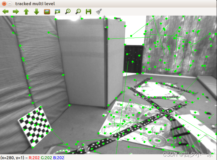
LK 光流跟踪能够直接得到特征点的对应关系。这个对应关系就像是描述子的匹配，只是光流对图像的连续性和光照稳定性要求更高一些。可以用光流跟踪的特征点，用 $P n P$ ， $I C P$ 或者对极几何来估计相机的运动。
总而言之，光流法可以加速基于特征点的视觉里程计算法，避免计算和匹配描述子的过程，但要求相机运动较为平滑(或者采集频率较高)。

相关阅读:
iptables详解：链、表、表链关系、规则的基本使用
python 科学计算三维可视化笔记（第一周基础运用）
Codeforces Round #833 (Div. 2）A — C
【华为上机考试真题】汽水瓶
用Speedtest-Tracker跟踪上网速度
虎扑论坛数据分析
使用ThreeJS绘制一个饼图
3.3 AOP之AOP概念及相关术语
干货分享｜一些好的数据分析、数据挖掘的网站或数据学习网站
【Linux】改变缓存路径、清理缓存

原文地址：https://blog.csdn.net/qq_35588369/article/details/124864242