使用 Python进行量化交易：前向验证分析

运行环境：Google Colab

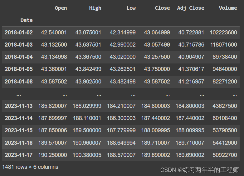
1. 利用 yfinance 下载数据

import yfinance as yf

ticker = 'AAPL'
df = yf.download(ticker)
df
1
2
3
4
5

• 下载苹果的股票数据

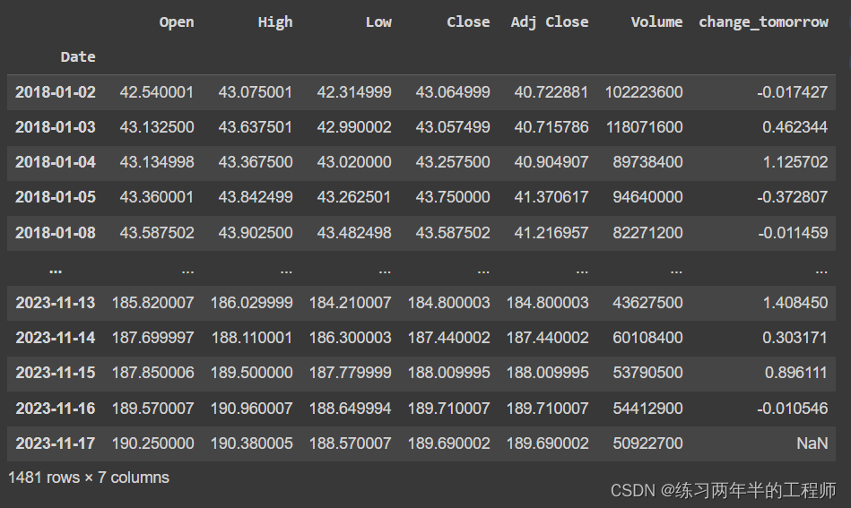
df = df.loc['2018-01-01':].copy()

df
1
2
3

df['change_tomorrow'] = df['Adj Close'].pct_change(-1)
df.change_tomorrow = df.change_tomorrow * -1
df.change_tomorrow = df.change_tomorrow * 100
df
1
2
3
4

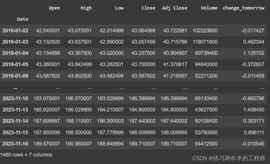
df = df.dropna().copy()
df
1
2

2. 变量准备

y = df.change_tomorrow
X = df[['Open','High','Low','Close','Volume']]
1
2

3. 时间序列数据的交叉验证

from sklearn.model_selection import TimeSeriesSplit

ts = TimeSeriesSplit(test_size=200)
1
2
3

• 使用了 Scikit-learn 库中的 TimeSeriesSplit 方法来创建时间序列交叉验证的实例。
• test_size=200 表示将数据集分成多个交叉验证折叠（folds），并且每个折叠的测试集大小为 200 个样本。

4. 随机森林回归模型来进行时间序列交叉验证

from sklearn.ensemble import RandomForestRegressor
from sklearn.metrics import mean_squared_error

model_dt = RandomForestRegressor(max_depth=15, random_state=42)

error_mse_list = []

for index_train, index_test in ts.split(df):
    X_train, y_train = X.iloc[index_train], y.iloc[index_train]
    X_test, y_test = X.iloc[index_test], y.iloc[index_test]
    
    model_dt.fit(X_train, y_train)
    
    y_pred = model_dt.predict(X_test)
    error_mse = mean_squared_error(y_test, y_pred)
    
    error_mse_list.append(error_mse)
1
2
3
4
5
6
7
8
9
10
11
12
13
14
15
16
17

• 使用之前创建的时间序列交叉验证实例 ts 在数据集 df 上进行拆分，index_train, index_test 是每次交叉验证的训练集和测试集的索引。
• 使用随机森林模型 model_dt 对训练集进行拟合。
• 使用训练好的模型对测试集的特征进行预测，得到预测结果 y_pred。
• 使用均方误差（MSE）方法，计算了真实值 y_test 和预测值 y_pred 之间的均方误差。

error_mse_list
1

[9.29226288135296,
6.621204525309144,
5.117431788350876,
5.570462756189788,
2.627530106136459]

5. 在每个交易周期根据模型的预测值执行买入或卖出操作

from backtesting import Backtest, Strategy
class Regression(Strategy):
    limit_buy = 1
    limit_sell = -5
    
    n_train = 600
    coef_retrain = 200
    
    def init(self):
        self.model = RandomForestRegressor(max_depth=15, random_state=42)
        self.already_bought = False
        
        X_train = self.data.df.iloc[:self.n_train, :-1]
        y_train = self.data.df.iloc[:self.n_train, -1]
        
        self.model.fit(X=X_train, y=y_train)

    def next(self):
        explanatory_today = self.data.df.iloc[[-1], :-1]
        forecast_tomorrow = self.model.predict(explanatory_today)[0]
        
        if forecast_tomorrow > self.limit_buy and self.already_bought == False:
            self.buy()
            self.already_bought = True
        elif forecast_tomorrow < self.limit_sell and self.already_bought == True:
            self.sell()
            self.already_bought = False
        else:
            pass
1
2
3
4
5
6
7
8
9
10
11
12
13
14
15
16
17
18
19
20
21
22
23
24
25
26
27
28
29

• limit_buy = 1 和 limit_sell = -5：买入和卖出的阈值。
• n_train = 600 和 coef_retrain = 200：用于模型训练的数据量和重新训练的频率。
• def next(self):: 这是每个交易周期调用的方法，用于执行具体的交易操作。

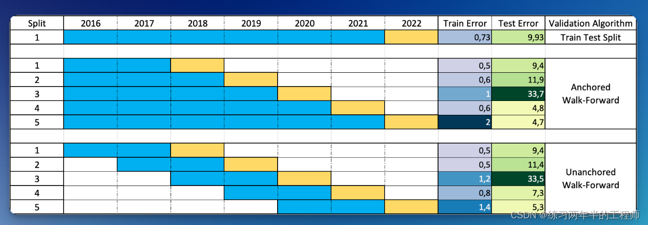
在前向优化中，回测数据被分成多个样本内和样本外段。策略在每个样本内段（蓝色）上进行优化，然后最优参数被应用到紧随其后的样本外段（黄色）。这种样本内优化和样本外测试的循环将随着整个数据集的进行而重复，形成一系列样本外回测。

Anchored Walk-Forward “锚定型”：样本内时间窗口始终从历史数据序列的开始开始，并逐步增加。

Unanchored Walk-Forward “非锚定型”：样本内时间窗口始终具有相同的持续时间，并且每个时间窗口都在前一个时间窗口之后开始。

6. 每经过一定时间后重新训练模型，以适应新的市场情况

class WalkForwardAnchored(Regression):
    def next(self):
        
        # we don't take any action and move on to the following day
        if len(self.data) < self.n_train:
            return
        
        # we retrain the model each 200 days
        if len(self.data) % self.coef_retrain == 0:
            X_train = self.data.df.iloc[:, :-1]
            y_train = self.data.df.iloc[:, -1]

            self.model.fit(X_train, y_train)

            super().next()
            
        else:
            
            super().next()
1
2
3
4
5
6
7
8
9
10
11
12
13
14
15
16
17
18
19

• if len(self.data) < self.n_train:: 这部分代码检查数据集长度是否小于预先设定的训练数据量 n_train。如果是，表示数据还不足以进行模型训练，于是不执行任何操作，直接跳转到下一个交易日。
• if len(self.data) % self.coef_retrain == 0:: 这部分代码检查当前数据长度是否达到了重新训练模型的时间节点（每经过 coef_retrain 天就重新训练一次模型）。
• 从当前数据集中重新获取特征集 X_train 和目标集 y_train。
• 使用这些数据重新训练模型 self.model。

from backtesting import Backtest
bt = Backtest(df, WalkForwardAnchored, cash=10000, commission=.002, exclusive_orders=True)
1
2

stats_skopt, heatmap, optimize_result = bt.optimize(
    limit_buy = range(0, 6), limit_sell = range(-6, 0),
    maximize='Return [%]',
    max_tries=500,
    random_state=42,
    return_heatmap=True,
    return_optimization=True,
    method='skopt'
    )

dff = heatmap.reset_index()
dff = dff.sort_values('Return [%]', ascending=False)
dff
1
2
3
4
5
6
7
8
9
10
11
12
13

7. 使用最近的 n_train 天数据作为训练集，从而保持模型更敏感地反映最近的市场情况

class WalkForwardUnanchored(Regression):
    def next(self):
        
        # we don't take any action and move on to the following day
        if len(self.data) < self.n_train:
            return
        
        # we retrain the model each 200 days
        if len(self.data) % self.coef_retrain == 0:
            X_train = self.data.df.iloc[-self.n_train:, :-1]
            y_train = self.data.df.iloc[-self.n_train:, -1]

            self.model.fit(X_train, y_train)

            super().next()
            
        else:
            
            super().next()
1
2
3
4
5
6
7
8
9
10
11
12
13
14
15
16
17
18
19

bt_unanchored = Backtest(df, WalkForwardUnanchored, cash=10000, commission=.002, exclusive_orders=True)

stats_skopt, heatmap, optimize_result = bt_unanchored.optimize(
    limit_buy = range(0, 6), limit_sell = range(-6, 0),
    maximize='Return [%]',
    max_tries=500,
    random_state=42,
    return_heatmap=True,
    return_optimization=True,
    method='skopt'
    )

dff = heatmap.reset_index()
dff = dff.sort_values('Return [%]', ascending=False)
dff
1
2
3
4
5
6
7
8
9
10
11
12
13
14
15