-
RCNN 目标检测网络学习笔记 (附代码)
论文地址:https://arxiv.org/abs/1311.2524
代码地址:https://github.com/rbgirshick/rcnn
1.是什么?
R-CNN系列论文(R-CNN,fast-RCNN,faster-RCNN)是使用深度学习进行物体检测的鼻祖论文,其中fast-RCNN 以及faster-RCNN都是沿袭R-CNN的思路。
R-CNN全称region with CNN features,其实它的名字就是一个很好的解释。用CNN提取出Region Proposals中的featues,然后进行SVM分类与bbox的回归。2.为什么?
RCNN是一种基于卷积神经网络的目标检测方法,相比于传统方法,它具有以下优势:
1. RCNN可以自动学习特征,不需要手工设计特征,因此可以更好地适应不同的场景和目标。
2. RCNN引入了候选区域的概念,可以减少搜索空间,提高检测速度。
3. RCNN可以同时检测多个目标,并且可以检测不同种类的目标。
4. RCNN在准确度和精度上都有很大提升,尤其是在复杂场景和目标不明显的情况下,相比传统方法更加准确。3.怎么样?
3.1网络结构
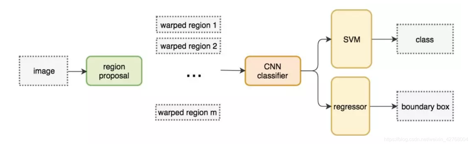
算法运行流程:
●找出图片中可能存在目标的侯选区域(region proposal)
●进行图片大小调整为了适应AlexNet网络的输入图像的大小227×227,通过CNN对候选区域提取特征向量,2000个建议框的CNN特征组合成2000×4096维矩阵
●将2000×4096维特征与20个SVM组成的权值矩阵4096×20相乘(20种分类,SVM是二分类器,则有20个SVM),获得2000×20维矩阵
●分别对2000×20维矩阵中每一列即每一类进行非极大值抑制(NMS:non-maximum suppression)剔除重叠建议框,得到该列即该类中得分最高的一些建议框
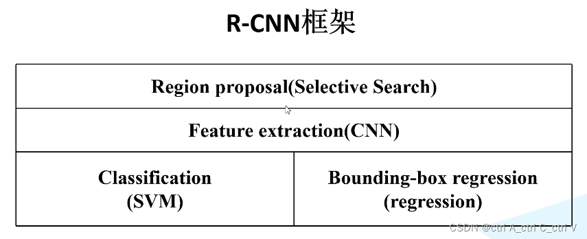
●修正Bounding box,对bbox做回归微调.3.2 框架
RCNN由四个部分组成:SS算法、CNN、SVM、bbox regression。
3.3 流程图

3.4 主要步骤
RCNN继承了传统目标检测的思想,将目标检测当做分类问题进行处理,先提取一系列目标的候选区域,然后对候选区域进行类。
其具体算法流程包含以下4步:
(1)生成候选区域:
采用一定区域候选算法(如 Selective Search)将图像分割成小区域,然后合并包含同一物体可能性高的区域作为候选区域输出,这里也需要采用一些合并策略。不同候选区域会有重合部分,如下图所示(黑色框是候选区域):

要生成1000-2000个候选区域(以2000个为例),之后将每个区域进行归一化,即缩放到固定的大小(227*227)
(2)对每个候选区域用CNN进行特征提取:
这里要事先选择一个预训练神经网络(如AlexNet、VGG),并重新训练全连接层,即 fintune 技术的应用。
将候选区域输入训练好的AlexNet CNN网络,得到固定维度的特征输出(4096维),得到2000×4096的特征矩阵。

(3)用每一类的SVM分类器对CNN的输出特征进行分类:
此处以PASCAL VOC数据集为例,该数据集中有20个类别,因此设置20个SVM分类器。
将 2000×4096 的特征与20个SVM组成的权值矩阵 4096×20 相乘,获得 2000×20 维的矩阵,表示2000个候选区域分别属于20个分类的概率,因此矩阵的每一行之和为1

非极大值抑制剔除重叠建议框的具体实现方法是:
第一步:定义 IoU 指数(Intersection over Union),即 (A∩B) / (AUB) ,即AB的重合区域面积与AB总面积的比。直观上来讲 IoU 就是表示AB重合的比率, IoU越大说明AB的重合部分占比越大,即A和B越相似。

第二步:找到每一类中2000个候选区域中概率最高的区域,计算其他区域与该区域的IoU值,删除所有IoU值大于阈值的候选区域。这样可以只保留少数重合率较低的候选区域,去掉重复区域。
比如下面的例子,A是向日葵类对应的所有候选框中概率最大的区域,B是另一个区域,计算AB的IoU,其结果大于阈值,那么就认为AB属于同一类(即都是向日葵),所以应该保留A,删除B,这就是非极大值抑制。

使用 SVM 进行二分类的一个问题是样本不均衡:背景图片很多,前景图片很少;导致 SVM 的训练需要解决样本不均衡的问题。
(4)使用回归器精修候选区域的位置:
通过 Selective Search算法得到的候选区域位置不一定准确,因此用20个回归器对上述20个类别中剩余的建议框进行回归操作,最终得到每个类别的修正后的目标区域。具体实现如下:
如图,黄色框表示候选区域 Region Proposal,绿色窗口表示实际区域Ground Truth(人工标注的),红色窗口表示 Region Proposal 进行回归后的预测区域,可以用最小二乘法解决线性回归问题。
通过回归器可以得到候选区域的四个参数,分别为:候选区域的x和y的偏移量,高度和宽度的缩放因子。可以通过这四个参数对候选区域的位置进行精修调整,就得到了红色的预测区域。

3.5 代码实现
- import os,cv2,keras
- import pandas as pd
- import matplotlib.pyplot as plt
- import numpy as np
- import tensorflow as tf
- path = "Images"
- annot = "Airplanes_Annotations"
- for e,i in enumerate(os.listdir(annot)):
- if e < 10:
- filename = i.split(".")[0]+".jpg"
- print(filename)
- img = cv2.imread(os.path.join(path,filename))
- df = pd.read_csv(os.path.join(annot,i))
- plt.imshow(img)
- for row in df.iterrows():
- x1 = int(row[1][0].split(" ")[0])
- y1 = int(row[1][0].split(" ")[1])
- x2 = int(row[1][0].split(" ")[2])
- y2 = int(row[1][0].split(" ")[3])
- cv2.rectangle(img,(x1,y1),(x2,y2),(255,0,0), 2)
- plt.figure()
- plt.imshow(img)
- break
- cv2.setUseOptimized(True);
- ss = cv2.ximgproc.segmentation.createSelectiveSearchSegmentation()
- im = cv2.imread(os.path.join(path,"42850.jpg"))
- ss.setBaseImage(im)
- ss.switchToSelectiveSearchFast()
- rects = ss.process()
- imOut = im.copy()
- for i, rect in (enumerate(rects)):
- x, y, w, h = rect
- # print(x,y,w,h)
- # imOut = imOut[x:x+w,y:y+h]
- cv2.rectangle(imOut, (x, y), (x+w, y+h), (0, 255, 0), 1, cv2.LINE_AA)
- # plt.figure()
- plt.imshow(imOut)
- train_images=[]
- train_labels=[]
- def get_iou(bb1, bb2):
- assert bb1['x1'] < bb1['x2']
- assert bb1['y1'] < bb1['y2']
- assert bb2['x1'] < bb2['x2']
- assert bb2['y1'] < bb2['y2']
- x_left = max(bb1['x1'], bb2['x1'])
- y_top = max(bb1['y1'], bb2['y1'])
- x_right = min(bb1['x2'], bb2['x2'])
- y_bottom = min(bb1['y2'], bb2['y2'])
- if x_right < x_left or y_bottom < y_top:
- return 0.0
- intersection_area = (x_right - x_left) * (y_bottom - y_top)
- bb1_area = (bb1['x2'] - bb1['x1']) * (bb1['y2'] - bb1['y1'])
- bb2_area = (bb2['x2'] - bb2['x1']) * (bb2['y2'] - bb2['y1'])
- iou = intersection_area / float(bb1_area + bb2_area - intersection_area)
- assert iou >= 0.0
- assert iou <= 1.0
- return iou
- ss = cv2.ximgproc.segmentation.createSelectiveSearchSegmentation()
- for e,i in enumerate(os.listdir(annot)):
- try:
- if i.startswith("airplane"):
- filename = i.split(".")[0]+".jpg"
- print(e,filename)
- image = cv2.imread(os.path.join(path,filename))
- df = pd.read_csv(os.path.join(annot,i))
- gtvalues=[]
- for row in df.iterrows():
- x1 = int(row[1][0].split(" ")[0])
- y1 = int(row[1][0].split(" ")[1])
- x2 = int(row[1][0].split(" ")[2])
- y2 = int(row[1][0].split(" ")[3])
- gtvalues.append({"x1":x1,"x2":x2,"y1":y1,"y2":y2})
- ss.setBaseImage(image)
- ss.switchToSelectiveSearchFast()
- ssresults = ss.process()
- imout = image.copy()
- counter = 0
- falsecounter = 0
- flag = 0
- fflag = 0
- bflag = 0
- for e,result in enumerate(ssresults):
- if e < 2000 and flag == 0:
- for gtval in gtvalues:
- x,y,w,h = result
- iou = get_iou(gtval,{"x1":x,"x2":x+w,"y1":y,"y2":y+h})
- if counter < 30:
- if iou > 0.70:
- timage = imout[y:y+h,x:x+w]
- resized = cv2.resize(timage, (224,224), interpolation = cv2.INTER_AREA)
- train_images.append(resized)
- train_labels.append(1)
- counter += 1
- else :
- fflag =1
- if falsecounter <30:
- if iou < 0.3:
- timage = imout[y:y+h,x:x+w]
- resized = cv2.resize(timage, (224,224), interpolation = cv2.INTER_AREA)
- train_images.append(resized)
- train_labels.append(0)
- falsecounter += 1
- else :
- bflag = 1
- if fflag == 1 and bflag == 1:
- print("inside")
- flag = 1
- except Exception as e:
- print(e)
- print("error in "+filename)
- continue
- X_new = np.array(train_images)
- y_new = np.array(train_labels)
- X_new.shape
- from keras.layers import Dense
- from keras import Model
- from keras import optimizers
- from keras.preprocessing.image import ImageDataGenerator
- from keras.applications.vgg16 import VGG16
- vggmodel = VGG16(weights='imagenet', include_top=True)
- vggmodel.summary()
- for layers in (vggmodel.layers)[:15]:
- print(layers)
- layers.trainable = False
- X= vggmodel.layers[-2].output
- predictions = Dense(2, activation="softmax")(X)
- model_final = Model(input = vggmodel.input, output = predictions)
- from keras.optimizers import Adam
- opt = Adam(lr=0.0001)
- model_final.compile(loss = keras.losses.categorical_crossentropy, optimizer = opt, metrics=["accuracy"])
- model_final.summary()
- from sklearn.model_selection import train_test_split
- from sklearn.preprocessing import LabelBinarizer
- class MyLabelBinarizer(LabelBinarizer):
- def transform(self, y):
- Y = super().transform(y)
- if self.y_type_ == 'binary':
- return np.hstack((Y, 1-Y))
- else:
- return Y
- def inverse_transform(self, Y, threshold=None):
- if self.y_type_ == 'binary':
- return super().inverse_transform(Y[:, 0], threshold)
- else:
- return super().inverse_transform(Y, threshold)
- lenc = MyLabelBinarizer()
- Y = lenc.fit_transform(y_new)
- X_train, X_test , y_train, y_test = train_test_split(X_new,Y,test_size=0.10)
- print(X_train.shape,X_test.shape,y_train.shape,y_test.shape)
- trdata = ImageDataGenerator(horizontal_flip=True, vertical_flip=True, rotation_range=90)
- traindata = trdata.flow(x=X_train, y=y_train)
- tsdata = ImageDataGenerator(horizontal_flip=True, vertical_flip=True, rotation_range=90)
- testdata = tsdata.flow(x=X_test, y=y_test)
- from keras.callbacks import ModelCheckpoint, EarlyStopping
- checkpoint = ModelCheckpoint("ieeercnn_vgg16_1.h5", monitor='val_loss', verbose=1, save_best_only=True, save_weights_only=False, mode='auto', period=1)
- early = EarlyStopping(monitor='val_loss', min_delta=0, patience=100, verbose=1, mode='auto')
- hist = model_final.fit_generator(generator= traindata, steps_per_epoch= 10, epochs= 1000, validation_data= testdata, validation_steps=2, callbacks=[checkpoint,early])
- import matplotlib.pyplot as plt
- # plt.plot(hist.history["acc"])
- # plt.plot(hist.history['val_acc'])
- plt.plot(hist.history['loss'])
- plt.plot(hist.history['val_loss'])
- plt.title("model loss")
- plt.ylabel("Loss")
- plt.xlabel("Epoch")
- plt.legend(["Loss","Validation Loss"])
- plt.show()
- plt.savefig('chart loss.png')
- im = X_test[1600]
- plt.imshow(im)
- img = np.expand_dims(im, axis=0)
- out= model_final.predict(img)
- if out[0][0] > out[0][1]:
- print("plane")
- else:
- print("not plane")
- z=0
- for e,i in enumerate(os.listdir(path)):
- if i.startswith("4"):
- z += 1
- img = cv2.imread(os.path.join(path,i))
- ss.setBaseImage(img)
- ss.switchToSelectiveSearchFast()
- ssresults = ss.process()
- imout = img.copy()
- for e,result in enumerate(ssresults):
- if e < 2000:
- x,y,w,h = result
- timage = imout[y:y+h,x:x+w]
- resized = cv2.resize(timage, (224,224), interpolation = cv2.INTER_AREA)
- img = np.expand_dims(resized, axis=0)
- out= model_final.predict(img)
- if out[0][0] > 0.65:
- cv2.rectangle(imout, (x, y), (x+w, y+h), (0, 255, 0), 1, cv2.LINE_AA)
- plt.figure()
- plt.imshow(imout)
4.然后捏!
R-CNN存在的问题
训练时间长:主要原因是分阶段多次训练,而且对于每个region proposal都要单独计算一次feature map,导致整体的时间变长。
占用空间大:每个region proposal的feature map都要写入硬盘中保存,以供后续的步骤使用。
multi-stage:文章中提出的模型包括多个模块,每个模块都是相互独立的,训练也是分开的。这会
导致精度不高,因为整体没有一个训练联动性,都是不共享分割训练的,自然最重要的CNN特征提取也不会做的太好。
测试时间长,由于不共享计算,所以对于test image,也要为每个proposal单独计算一次feature map,因此测试时间也很长。
-
相关阅读:
Linux:syslog()的使用和示例
C语言操作符深度解析(四)
使用boost封装一个websocketserver类
利用Nextcloud搭建企业私有云盘系统
【Java】IO流体常用类FileReader和FileWriter
图像特征算法---ORB算法的python实现
原来电商企业也能运用模型规划设计营销活动
STM32--基于STM32的智能家居设计与实现
ICMPv6与NDP
虚幻4学习笔记(11) 蓝图实现AI移动、AI树实现移动、看见后寻找玩家
- 原文地址:https://blog.csdn.net/PLANTTHESON/article/details/134049926
