cartographer中的扫描匹配

cartographer中的扫描匹配

cartographer中使用了两种扫描匹配方法：CSM（相关性扫描匹配方法（暴力匹配））、ceres优化匹配方法

CSM可以简单地理解为暴力搜索，即每一个激光数据与子图里的每一个位姿进行匹配，直到找到最优位姿，进行三层for循环，不过谷歌采用多分辨率搜索的方式，来降低计算量。基于优化的方法是谷歌的ceres库来实现，原理就是构造误差函数，使其对最小化，其精度高，但是对初始值敏感。

扫描匹配在cartographer中的调用

在cartographer的前端local_trajectory_builder_2d中会对传入的点云数据做各种处理，在对点云数据进行体素滤波之后传给ScanMatch进行扫描匹配。

// 扫描匹配, 进行点云与submap的匹配
std::unique_ptr pose_estimate_2d =
   ScanMatch(time, pose_prediction, filtered_gravity_aligned_point_cloud);
1
2
3

ScanMatch函数中调用real_time_correlative_scan_matcher_.Match函数进行相关性扫描匹配

​ 调用ceres_scan_matcher_.Match函数使用ceres优化匹配

// 根据参数决定是否 使用correlative_scan_matching对先验位姿进行校准
  if (options_.use_online_correlative_scan_matching()) {
    const double score = real_time_correlative_scan_matcher_.Match(
        pose_prediction, filtered_gravity_aligned_point_cloud,
        *matching_submap->grid(), &initial_ceres_pose);
    kRealTimeCorrelativeScanMatcherScoreMetric->Observe(score);
  }

  auto pose_observation = absl::make_unique();
  ceres::Solver::Summary summary;
  // 使用ceres进行扫描匹配
  ceres_scan_matcher_.Match(pose_prediction.translation(), initial_ceres_pose,
                            filtered_gravity_aligned_point_cloud,
                            *matching_submap->grid(), pose_observation.get(),
                            &summary);
1
2
3
4
5
6
7
8
9
10
11
12
13
14
15

ScanMatch函数

ScanMatch需要传入的参数：

time //点云时间
pose_prediction //先验位姿
filtered_gravity_aligned_point_cloud //匹配用的点云
1
2
3

ScanMatch返回值：

std::unique_ptr //匹配后的二维位姿
1

首先判断submaps是否为空，为空的话直接返回传入的先验位姿pose_prediction

if (active_submaps_.submaps().empty()) {
  return absl::make_unique(pose_prediction);
}
1
2
3

不为空，向下继续执行

将submaps的第一个子图赋值给matching_submap，用于匹配

std::shared_ptr matching_submap =
   active_submaps_.submaps().front();
1
2

将传入的先验位姿赋值给matching_submap，作为ceres优化匹配的初始位姿

std::shared_ptr matching_submap =
    active_submaps_.submaps().front();
1
2

根据配置文件的use_online_correlative_scan_matching参数，选择是否使用相关性匹配对先验位姿进行校准。

配置参数在src/cartographer/configuration_files/trajectory_builder_2d.lua文件中

-- 是否使用 real_time_correlative_scan_matcher 为ceres提供先验信息
  -- 计算复杂度高 , 但是很鲁棒 , 在odom或者imu不准时依然能达到很好的效果
  use_online_correlative_scan_matching = false,
  real_time_correlative_scan_matcher = {
    linear_search_window = 0.1,             -- 线性搜索窗口的大小
    angular_search_window = math.rad(20.),  -- 角度搜索窗口的大小
    -- 用于计算各部分score的权重
    translation_delta_cost_weight = 1e-1,   -- 平移
    rotation_delta_cost_weight = 1e-1,      -- 旋转
  },
1
2
3
4
5
6
7
8
9
10

若use_online_correlative_scan_matching参数选择为TRUE，就调用real_time_correlative_scan_matcher_.Match函数，进行相关性扫描匹配，校准先验位姿，返回的是匹配得分

if (options_.use_online_correlative_scan_matching()) {
  const double score = real_time_correlative_scan_matcher_.Match(
      pose_prediction, filtered_gravity_aligned_point_cloud,
      *matching_submap->grid(), &initial_ceres_pose);
  kRealTimeCorrelativeScanMatcherScoreMetric->Observe(score);
}
1
2
3
4
5
6

若use_online_correlative_scan_matching参数选择为FALSE，则直接使用传入的先验位姿pose_prediction作为ceres优化的初始位姿，调用ceres_scan_matcher_.Match函数进行ceres优化匹配

auto pose_observation = absl::make_unique();
  ceres::Solver::Summary summary;
  // 使用ceres进行扫描匹配
  ceres_scan_matcher_.Match(pose_prediction.translation(), initial_ceres_pose,
                            filtered_gravity_aligned_point_cloud,
                            *matching_submap->grid(), pose_observation.get(),
                            &summary);
1
2
3
4
5
6
7

相关性扫描匹配

相关性扫描匹配方法实现在real_time_correlative_scan_matcher_.Match这个函数

传入参数：

initial_pose_estimate //预测出来的先验位姿
point_cloud //用于匹配的点云 点云的原点位于local坐标系原点
grid //用于匹配的栅格地图
1
2
3

输出的参数：

pose_estimate //校正后的位姿
1

返回值：

double  best_candidate.score  //匹配得分
1

代码步骤：

1. 将点云旋转到预测的方向上
2. 生成按照不同角度旋转后的点云集合
3. 将旋转后的点云集合按照预测出的平移量进行平移，获取平移后的点在地图中的索引
4. 生成所有的候选解
5. 计算所有候选解的加权得分
6. 获取最优解
7. 将计算出的偏差量加上原始位姿获得校正后的位姿

step1. 将点云旋转到预测的方向上

传入的点云是经过变换到local坐标系原点的点云数据，需要将传入的点云数据进行旋转变换，变换到预测的方向上。

//获取初始位姿的角度即旋转量
const Eigen::Rotation2Dd initial_rotation = initial_pose_estimate.rotation();
//将点云数据进行坐标变换
const sensor::PointCloud rotated_point_cloud = sensor::TransformPointCloud(
    point_cloud,
    transform::Rigid3f::Rotation(Eigen::AngleAxisf(
        initial_rotation.cast().angle(), Eigen::Vector3f::UnitZ())));
1
2
3
4
5
6
7

根据配置参数初始化 SearchParameters数据结构，定义搜索的空间，包括平移的窗口和角度窗口

const SearchParameters search_parameters(
    options_.linear_search_window(), options_.angular_search_window(),
    rotated_point_cloud, grid.limits().resolution());
1
2
3

参数还是前面说的那个配置文件中

这里是调用了SearchParameters的构造函数，进入SearchParameters的构造函数

 // 求得 point_cloud 中雷达数据的 最大的值（最远点的距离）
  for (const sensor::RangefinderPoint& point : point_cloud) {
    const float range = point.position.head<2>().norm();
    max_scan_range = std::max(range, max_scan_range);
  }
1
2
3
4
5

计算论文中提到的角度分辨率

其中：d是雷达的最远距离，r是栅格的分辨率

求θ

根据余弦定理：
$$cos\theta =\frac{b^2+c^2-a^2}{2bc}$$
则有
$$
cosθ = \frac{d^2 + d^2 - r^2}{2dd}

 = 1 - \frac{r^2}{2d^2}
1

$$即$$
θ = arccos(1-\frac{r^2}{2d2})
$$

// 根据论文里的公式 求得角度分辨率 angular_perturbation_step_size
const double kSafetyMargin = 1. - 1e-3;
angular_perturbation_step_size =
    kSafetyMargin * std::acos(1. - common::Pow2(resolution) /
                                       (2. * common::Pow2(max_scan_range)));
1
2
3
4
5

根据传入的角度搜索窗除以角度分辨率，就能够得到划分的角度个数范围

// 范围除以分辨率得到个数
num_angular_perturbations =
    std::ceil(angular_search_window / angular_perturbation_step_size);
1
2
3

将划分得到的角度个数范围扩大2倍再加1，得到要生成的旋转点云的个数。划分得到的角度个数是一个正数，点云会从他的负的最小开始算，所以会乘以2倍，还有0所以会加1，就是点云的个数。

num_scans = 2 * num_angular_perturbations + 1;
1

用传入的线性搜索窗除以分辨率可以得到xy方向的搜索范围，单位是栅格

const int num_linear_perturbations =
    std::ceil(linear_search_window / resolution);
1
2

确定每一个点云的最大最小边界

linear_bounds.reserve(num_scans);
for (int i = 0; i != num_scans; ++i) {
  linear_bounds.push_back(
      LinearBounds{-num_linear_perturbations, num_linear_perturbations,
                   -num_linear_perturbations, num_linear_perturbations});
1
2
3
4
5

step2. 生成按照不同角度旋转后的点云集合

const std::vector rotated_scans =
    GenerateRotatedScans(rotated_point_cloud, search_parameters);
1
2

search_parameters存了需要旋转的点云的个数num_scans，乘以角分辨率之后就是不同的角度

进入GenerateRotatedScans函数

首先计算起始角度，划分得到的角度范围num_angular_perturbations是从负值到正值的，起始位置就从负的最小角开始，再乘以分辨率得到需要的角度

double delta_theta = -search_parameters.num_angular_perturbations *
                     search_parameters.angular_perturbation_step_size;
1
2

最后进行遍历，生成旋转不同角度后的点云集合

for (int scan_index = 0; scan_index < search_parameters.num_scans;
     ++scan_index,
         delta_theta += search_parameters.angular_perturbation_step_size) {
  // 将 point_cloud 绕Z轴旋转了delta_theta
  rotated_scans.push_back(sensor::TransformPointCloud(
      point_cloud, transform::Rigid3f::Rotation(Eigen::AngleAxisf(
                       delta_theta, Eigen::Vector3f::UnitZ()))));
}
1
2
3
4
5
6
7
8

step3. 将旋转后的点云集合按照预测出的平移量进行平移, 获取平移后的点在地图中的索引

const std::vector discrete_scans = DiscretizeScans(
    grid.limits(), rotated_scans,
    Eigen::Translation2f(initial_pose_estimate.translation().x(),
                         initial_pose_estimate.translation().y()));
1
2
3
4

调用DiscretizeScans函数，将旋转后的点云集合按照预测出的平移量进行平移，获取平移后的点在地图中的索引

先定义一个DiscreteScan2D结构的变量 discrete_scans，用于存放平移后的点云在地图中的索引

然后申请相应点云数量的空间

std::vector discrete_scans;
discrete_scans.reserve(scans.size());
1
2

进入第一层for循环，遍历每一个角度的点云

for (const sensor::PointCloud& scan : scans) {
    // discrete_scans中的每一个 DiscreteScan2D 的size设置为这一帧点云中所有点的个数
    discrete_scans.emplace_back();
    discrete_scans.back().reserve(scan.size());
    ...}
1
2
3
4
5

进入第二层for循环，对点云中的每个点进行平移，获取平移后的栅格索引

for (const sensor::RangefinderPoint& point : scan) {
    // 对scan中的每个点进行平移
    const Eigen::Vector2f translated_point =
        Eigen::Affine2f(initial_translation) * point.position.head<2>();

    // 将平移后的点 对应的栅格的索引放入discrete_scans
    discrete_scans.back().push_back(
        map_limits.GetCellIndex(translated_point));
    }
1
2
3
4
5
6
7
8
9

通过point.position.head<2>取出点云的x，y坐标，然后乘以一个平移量Affine2f(initial_translation)，对这个点进行平移。

const Eigen::Vector2f translated_point =
      Eigen::Affine2f(initial_translation) * point.position.head<2>();
1
2

通过平移后的点的坐标传入GetCellIndex函数，获得物理坐标在栅格地图中的栅格的索引

map_limits.GetCellIndex(translated_point));
1

最后返回平移后的点在地图中的索引

return discrete_scans
1

step4. 生成所有的候选解

std::vector candidates =
    GenerateExhaustiveSearchCandidates(search_parameters);
1
2

进入GenerateExhaustiveSearchCandidates函数，首先获取所有候选解的个数

遍历经过旋转后的所有角度的点云，判断每一个角度上的点云会有多少种可能性，将其记录到num_candidates中。

首先计算x坐标上的点数，然后计算对应y坐标上的点数，将x乘以y得到总的可能性。

举例说明，假设栅格中的一个点在x方向有十个栅格的的距离，在y方向上有五个栅格的距离，那么他总共可平移的栅格就是50个，然后总共有8个点，那么所有的平移栅格就是400个。

for (int scan_index = 0; scan_index != search_parameters.num_scans;
     ++scan_index) {
  const int num_linear_x_candidates =
      (search_parameters.linear_bounds[scan_index].max_x -
       search_parameters.linear_bounds[scan_index].min_x + 1);
  const int num_linear_y_candidates =
      (search_parameters.linear_bounds[scan_index].max_y -
       search_parameters.linear_bounds[scan_index].min_y + 1);
  num_candidates += num_linear_x_candidates * num_linear_y_candidates;
}
1
2
3
4
5
6
7
8
9
10

然后生成候选解，首先遍历所有角度的点云个数，然后遍历所有的点云的x坐标，最后遍历每个x偏移量，y偏移量，最后将点云索引，x坐标，y坐标，配置参数传给 candidates 生成所有的候选解。

for (int scan_index = 0; scan_index != search_parameters.num_scans;
     ++scan_index) {
  for (int x_index_offset = search_parameters.linear_bounds[scan_index].min_x;
       x_index_offset <= search_parameters.linear_bounds[scan_index].max_x;
       ++x_index_offset) {
    for (int y_index_offset =
             search_parameters.linear_bounds[scan_index].min_y;
         y_index_offset <= search_parameters.linear_bounds[scan_index].max_y;
         ++y_index_offset) {
      candidates.emplace_back(scan_index, x_index_offset, y_index_offset,
                              search_parameters);
    }
  }
}
1
2
3
4
5
6
7
8
9
10
11
12
13
14

最后检查得到的候选解的size是否等于候选解的个数num_candidates，相等就返回所有候选解

CHECK_EQ(candidates.size(), num_candidates);
return candidates;
1
2

step5. 计算所有候选解得加权得分

ScoreCandidates(grid, discrete_scans, search_parameters, &candidates);
1

进入ScoreCandidates函数

遍历所有候选解，判断传入的地图类型（栅格地图（PROBABILITY_GRID）或三维点云地图（TSDF））

将点云在栅格地图中的索引，x、y的偏移量传给ComputeCandidateScore函数，计算每个栅格的得分。

for (Candidate2D& candidate : *candidates) {
  switch (grid.GetGridType()) {
    case GridType::PROBABILITY_GRID:
      candidate.score = ComputeCandidateScore(
          static_cast(grid),
          discrete_scans[candidate.scan_index], candidate.x_index_offset,
          candidate.y_index_offset);
      break;
1
2
3
4
5
6
7
8

进入ComputeCandidateScore函数

遍历点云在栅格地图中的xy坐标，加上xy的偏移量得到点云的平移和旋转之后的在栅格地图中的坐标

for (const Eigen::Array2i& xy_index : discrete_scan) {
    // 对每个点都加上像素坐标的offset, 相当于对点云进行平移
    const Eigen::Array2i proposed_xy_index(xy_index.x() + x_index_offset,
                                           xy_index.y() + y_index_offset);
1
2
3
4

获取平移后的点云在栅格中占用的概率

const float probability =
      probability_grid.GetProbability(proposed_xy_index);
1
2

将获得的所有点的占用概率累加，得到此候选解得概率得分

  candidate_score += probability;
  }
1
2

将累加得分除以点的个数，获得此候选解的平均得分，并返回

candidate_score /= static_cast(discrete_scan.size());
CHECK_GT(candidate_score, 0.f);
return candidate_score;
1
2
3

最后回到ScoreCandidates函数，对每个得分根据参数配置的平移和旋转的权重进行加权

candidate.score *=
      std::exp(-common::Pow2(std::hypot(candidate.x, candidate.y) *
                                 options_.translation_delta_cost_weight() +
                             std::abs(candidate.orientation) *
                                 options_.rotation_delta_cost_weight()));
1
2
3
4
5

step6. 获取最优解

使用std::max_element获取候选解中得分最高的一组最为最优解

const Candidate2D& best_candidate =
    *std::max_element(candidates.begin(), candidates.end());
1
2

step7. 将计算出的偏差量加上原始位姿获得校正后的位姿

*pose_estimate = transform::Rigid2d(
    {initial_pose_estimate.translation().x() + best_candidate.x,
     initial_pose_estimate.translation().y() + best_candidate.y},
    initial_rotation * Eigen::Rotation2Dd(best_candidate.orientation));
return best_candidate.score;
1
2
3
4
5

基于ceres的扫描匹配

ceres基本原理

基于ceres的扫描匹配（即非线性优化）的实现在ceres_scan_matcher_.Match函数，代码文件位置：src/cartographer/cartographer/mapping/internal/2d/scan_matching/ceres_scan_matcher_2d.cc、.h

CreateCeresScanMatcherOptions2D的构造函数主要是对配置文件中的参数进行读取，主要还是在CeresScanMatcher2D类中实现。类CeresScanMatcher2D只定义了两个成员变量。 其中，options_ 用于记录扫描匹配器的相关配置，而变量ceres_solver_options_则是优化过程的配置。

CeresScanMatcher2D类的核心就在于Match这个函数的实现，这个函数的目的就是扫描匹配

在给定机器人的初始位姿估计initial_pose_estimate的情况下，尽可能的将扫描的点云数据point_cloud放置到栅格地图grid上， 同时返回优化后的位姿估计pose_estimate和优化迭代信息summary。而参数target_translation主要用于约束位姿估计的xy坐标， 在Local SLAM的业务主线调用该函数的时候传递的是位姿估计器的估计值，Cartographer认为优化后的机器人位置应当与该估计值的偏差不大。

输入参数：

 * @param[in] target_translation 预测出来的先验位置, 只有xy
 * @param[in] initial_pose_estimate (校正后的)先验位姿, 有xy与theta
 * @param[in] point_cloud 用于匹配的点云 点云的原点位于local坐标系原点
 * @param[in] grid 用于匹配的栅格地图
1
2
3
4

输出参数：

 * @param[out] pose_estimate 优化之后的位姿
 * @param[out] summary 优化迭代信息
1
2

首先是创建一个double数组，用于存放输入的初始位姿x，y和θ，然后创建一个problem的对象用于描述将要求解的问题。

double ceres_pose_estimate[3] = {initial_pose_estimate.translation().x(),
                                 initial_pose_estimate.translation().y(),
                                 initial_pose_estimate.rotation().angle()};
ceres::Problem problem;
1
2
3
4

然后就是描述地图、平移和旋转的残差，在配置文件中为这三类来源定义了权重。

CHECK_GT(options_.occupied_space_weight(), 0.);
problem.AddResidualBlock(
    CreateOccupiedSpaceCostFunction2D(
        options_.occupied_space_weight() /
            std::sqrt(static_cast(point_cloud.size())),
        point_cloud, grid),
    nullptr /* loss function */, ceres_pose_estimate);

CHECK_GT(options_.translation_weight(), 0.);
problem.AddResidualBlock(
    TranslationDeltaCostFunctor2D::CreateAutoDiffCostFunction(
        options_.translation_weight(), target_translation), // 平移的目标值, 没有使用校准后的平移（这里可能有点问题）
    nullptr /* loss function */, ceres_pose_estimate);      // 平移的初值

  // 旋转的残差, 固定了角度不变
CHECK_GT(options_.rotation_weight(), 0.);
problem.AddResidualBlock(
    RotationDeltaCostFunctor2D::CreateAutoDiffCostFunction(
        options_.rotation_weight(), ceres_pose_estimate[2]), // 角度的目标值
    nullptr /* loss function */, ceres_pose_estimate);       // 角度的初值

1
2
3
4
5
6
7
8
9
10
11
12
13
14
15
16
17
18
19
20
21

Cartographer为三类不同的残差源分别定义了一个类，并通过其静态函数CreateAutoDiffCostFunction提供使用Ceres原生的自动求导方法的代价函数计算。

通过其中RotationDeltaCostFunctor2D类来看看CreateAutoDiffCostFunction这个函数的实现

CreateAutoDiffCostFunction是类RotationDeltaCostFunctor2D公开的静态成员。有两个参数，其中scaling_factor是角度偏差的权重，可以通过配置文件指定; target_angle则是参考角度， 实际的调用传参是优化之前的角度估计。该函数最终构造和返回的是Ceres的AutoDiffCostFunction对象，从第2行中的模板列表中可以看到类RotationDeltaCostFunctor2D只提供一个残差项，其参与优化的参数有3个。

class RotationDeltaCostFunctor2D {
 public:
  // 静态成员函数, 返回CostFunction
  static ceres::CostFunction* CreateAutoDiffCostFunction(
      const double scaling_factor, const double target_angle) {
    return new ceres::AutoDiffCostFunction<
        RotationDeltaCostFunctor2D, 1 /* residuals */, 3 /* pose variables */>(
        new RotationDeltaCostFunctor2D(scaling_factor, target_angle));
  }
1
2
3
4
5
6
7
8
9

template 
bool operator()(const T* const pose, T* residual) const {
  residual[0] = scaling_factor_ * (pose[2] - angle_);
  return true; 
}
1
2
3
4
5

左边是类RotationDeltaCostFunctor2D对运算符"()"的重载，在第四行中计算角度偏差量并乘上权重得到残差项的代价。 这里的scaling_factor_和angle_是在类RotationDeltaCostFunctor2D中定义的两个私有成员变量分别记录了权重和参考角度。它们通过构造函数和静态函数CreateAutoDiffCostFunction的传参赋值。

类TranslationDeltaCostFunctor2D和OccupiedSpaceCostFunction2D也是以相同的套路实现的，把构造函数定义成私有的，防止用户直接构造对象。 在静态函数CreateAutoDiffCostFunction中以这两个类型为基础构建AutoDiffCostFunction对象。类TranslationDeltaCostFunctor2D定义了成员变量x_和y_用于记录位移偏差量的参考坐标。 类OccupiedSpaceCostFunction2D则使用成员变量point_cloud_和grid_分别记录待匹配的激光点云数据和栅格地图。

左边是类TranslationDeltaCostFunctor2D对运算符"()"的重载，它有两个残差项的代价需要计算，分别对应着x轴和y轴上的偏差量。在第4,5行中计算位置偏差量并乘上权重（尺度因子）来更新对应残差项的代价。

// 平移量残差的计算, (pose[0] - x_)的平方ceres会自动加上
template 
bool operator()(const T* const pose, T* residual) const {
  residual[0] = scaling_factor_ * (pose[0] - x_);
  residual[1] = scaling_factor_ * (pose[1] - y_);
  return true;
}
1
2
3
4
5
6
7

这里计算残差，都是基于使用的传感器预测的位姿很准的情况。

所以在调参的时候，如果传感器不是很好，位姿估计器不准确，可以适当的将地图的权重调的大于平移和旋转的权重。若是调参一直调不好，可以将计算平移和旋转的残差注释掉。

最后看看地图部分的残差

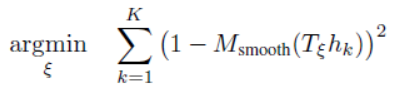
同样也是通过CreateAutoDiffCostFunction函数构建costFunction，他的构造是将地图的权重除以点云的数量，得到一个平均值，然后再进行传入，所以地图的权重就会被分散，当点云的数量越来越多时，地图的权重就会被分散的越来越小。

problem.AddResidualBlock(
        CreateOccupiedSpaceCostFunction2D(
            options_.occupied_space_weight() /
                std::sqrt(static_cast(point_cloud.size())),
            point_cloud, grid),
        nullptr /* loss function */, ceres_pose_estimate);
1
2
3
4
5
6

下面是类OccupiedSpaceCostFunction2D对运算符"()"的重载。在函数的一开始，先把迭代查询的输入参数pose转换为坐标变换Tε用临时变量transform记录。

template 
bool operator()(const T* const pose, T* residual) const {
  Eigen::Matrix translation(pose[0], pose[1]);
  Eigen::Rotation2D rotation(pose[2]);
  Eigen::Matrix rotation_matrix = rotation.toRotationMatrix();
  Eigen::Matrix transform;
  transform << rotation_matrix, translation, T(0.), T(0.), T(1.);
1
2
3
4
5
6
7

然后使用Ceres库原生提供的双三次插值迭代器。

const GridArrayAdapter adapter(grid_);
ceres::BiCubicInterpolator interpolator(adapter);
const MapLimits& limits = grid_.limits();
1
2
3

针对每个hit点计算对应的残差代价。

for (size_t i = 0; i < point_cloud_.size(); ++i) {
  // Note that this is a 2D point. The third component is a scaling factor.
  const Eigen::Matrix point((T(point_cloud_[i].position.x())),
                                     (T(point_cloud_[i].position.y())),
                                     T(1.));
  // 根据预测位姿对单个点进行坐标变换
  const Eigen::Matrix world = transform * point;
  // 获取三次插值之后的栅格free值, Evaluate函数内部调用了GetValue函数
  interpolator.Evaluate(
      (limits.max().x() - world[0]) / limits.resolution() - 0.5 +
          static_cast(kPadding),
      (limits.max().y() - world[1]) / limits.resolution() - 0.5 +
          static_cast(kPadding),
      &residual[i]);
  // free值越小, 表示占用的概率越大
  residual[i] = scaling_factor_ * residual[i];
}
1
2
3
4
5
6
7
8
9
10
11
12
13
14
15
16
17

参考：https://gaoyichao.com/Xiaotu/?book=Cartographer%E6%BA%90%E7%A0%81%E8%A7%A3%E8%AF%BB&title=%E5%9F%BA%E4%BA%8ECeres%E5%BA%93%E7%9A%84%E6%89%AB%E6%8F%8F%E5%8C%B9%E9%85%8D%E5%99%A8

使用ceres优化扫描匹配，除了要求hit点在占用栅格上出现的概率最大化之外， 还通过两个残差项约束了优化后的位姿估计在原始估计的附近。

总结

cartographer中使用了两种扫描匹配方法：CSM（相关性扫描匹配方法（暴力匹配））、ceres优化匹配方法

CSM可以简单地理解为暴力搜索，即每一个激光数据与子图里的每一个位姿进行匹配，直到找到最优位姿，进行三层for循环，不过谷歌采用多分辨率搜索的方式，来降低计算量。基于优化的方法是谷歌的ceres库来实现，原理就是构造误差函数，使其对最小化，其精度高，但是对初始值敏感。

在cartographer的前端local_trajectory_builder_2d中会对传入的点云数据做各种处理，在对点云数据进行体素滤波之后传给ScanMatch进行扫描匹配。

// 扫描匹配, 进行点云与submap的匹配
std::unique_ptr pose_estimate_2d =
   ScanMatch(time, pose_prediction, filtered_gravity_aligned_point_cloud);
1
2
3

ScanMatch函数中调用real_time_correlative_scan_matcher_.Match函数进行相关性扫描匹配

eres%E5%BA%93%E7%9A%84%E6%89%AB%E6%8F%8F%E5%8C%B9%E9%85%8D%E5%99%A8

使用ceres优化扫描匹配，除了要求hit点在占用栅格上出现的概率最大化之外， 还通过两个残差项约束了优化后的位姿估计在原始估计的附近。