Transformer和BERT可谓是LLM的基础模型,彻底搞懂极其必要。Transformer最初设想是作为文本翻译模型使用的,而BERT模型构建使用了Transformer的部分组件,如果理解了Transformer,则能很轻松地理解BERT。
一.Transformer模型架构
 1.编码器
1.编码器
(1)Multi-Head Attention(多头注意力机制)
首先将输入x进行embedding编码,然后通过WQ、WK和WV矩阵转换为Q、K和V,然后输入Scaled Dot-Product Attention中,最后经过Feed Forward输出,作为解码器第2层的输入Q。
(2)Feed Forward(前馈神经网络)
2.解码器
(1)Masked Multi-Head Attention(掩码多头注意力机制)
Masked包括上三角矩阵Mask(不包含对角线)和PAD MASK的叠加,目的是在计算自注意力过程中不会注意当前词的下一个词,只会注意当前词与当前词之前的词。在模型训练的时候为了防止误差积累和并行训练,使用Teacher Forcing机制。
(2)Encoder-Decoder Multi-Head Attention(编解码多头注意力机制)
把Encoder的输出作为解码器第2层的Q,把Decoder第1层的输出作为K和V。
(3)Feed Forward(前馈神经网络)
二.简单翻译任务
1.定义数据集
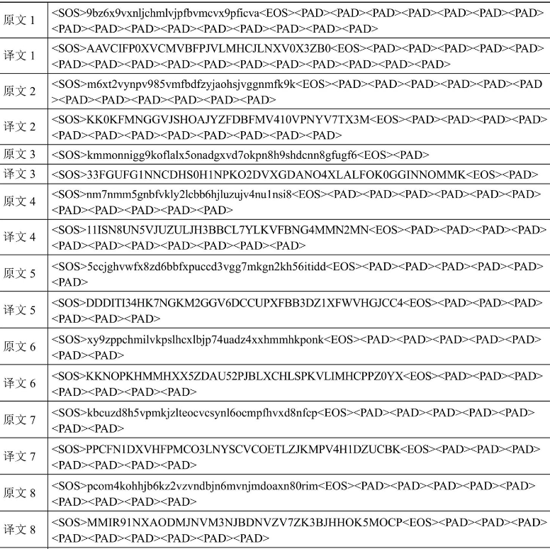
这块简要介绍,主要是通过数据生成器模拟了一些数据,将原文翻译为译文,实现代码如下所示:
# 定义字典
vocab_x = ',,,0,1,2,3,4,5,6,7,8,9,q,w,e,r,t,y,u,i,o,p,a,s,d,f,g,h,j,k,l,z,x,c,v,b,n,m'
vocab_x = {word: i for i, word in enumerate(vocab_x.split(','))}
vocab_xr = [k for k, v in vocab_x.items()]
vocab_y = {k.upper(): v for k, v in vocab_x.items()}
vocab_yr = [k for k, v in vocab_y.items()]
print('vocab_x=', vocab_x)
print('vocab_y=', vocab_y)
# 定义生成数据的函数
def get_data():
# 定义词集合
words =['0','1','2','3','4','5','6','7','8','9','q','w','e','r','t','y','u','i','o','p','a','s','d','f','g','h','j','k','l','z','x','c','v','b','n','m']
# 定义每个词被选中的概率
p = np.array([
1, 2, 3, 4, 5, 6, 7, 8, 9, 10, 1, 2, 3, 4, 5, 6, 7, 8, 9, 10, 11, 12,
13, 14, 15, 16, 17, 18, 19, 20, 21, 22, 23, 24, 25, 26
])
p = p / p.sum()
# 随机选n个词
n = random.randint(30, 48) # 生成30-48个词
x = np.random.choice(words, size=n, replace=True, p=p) # words中选n个词,每个词被选中的概率为p,replace=True表示可以重复选择
# 采样的结果就是x
x = x.tolist()
# y是由对x的变换得到的
# 字母大写,数字取9以内的互补数
def f(i):
i = i.upper()
if not i.isdigit():
return i
i = 9 - int(i)
return str(i)
y = [f(i) for i in x]
# 逆序
y = y[::-1]
# y中的首字母双写
y = [y[0]] + y
# 加上首尾符号
x = ['' ] + x + ['' ]
y = ['' ] + y + ['' ]
# 补PAD,直到固定长度
x = x + ['' ] * 50
y = y + ['' ] * 51
x = x[:50]
y = y[:51]
# 编码成数据
x = [vocab_x[i] for i in x]
y = [vocab_y[i] for i in y]
# 转Tensor
x = torch.LongTensor(x)
y = torch.LongTensor(y)
return x, y
# 定义数据集
class Dataset(torch.utils.data.Dataset):
def __init__(self): # 初始化
super(Dataset, self).__init__()
def __len__(self): # 返回数据集的长度
return 1000
def __getitem__(self, i): # 根据索引返回数据
return get_data()
然后通过loader = torch.utils.data.DataLoader(dataset=Dataset(), batch_size=8, drop_last=True, shuffle=True, collate_fn=None)定义了数据加载器,数据样例如下所示:
2.定义PAD MASK函数
PAD MASK主要目的是减少计算量,如下所示:
def mask_pad(data):
# b句话,每句话50个词,这里是还没embed的
# data = [b, 50]
# 判断每个词是不是' ]
# [b, 50] -> [b, 1, 1, 50]
mask = mask.reshape(-1, 1, 1, 50)
# 在计算注意力时,计算50个词和50个词相互之间的注意力,所以是个50*50的矩阵
# PAD的列为True,意味着任何词对PAD的注意力都是0,但是PAD本身对其它词的注意力并不是0,所以是PAD的行不为True
# 复制n次
# [b, 1, 1, 50] -> [b, 1, 50, 50]
mask = mask.expand(-1, 1, 50, 50) # 根据指定的维度扩展
return mask
if __name__ == '__main__':
# 测试mask_pad函数
print(mask_pad(x[:1]))
输出结果shape为(1,1,50,50)如下所示:
tensor([[[[False, False, False,  ..., False, False,  True],
          [False, False, False,  ..., False, False,  True],
          [False, False, False,  ..., False, False,  True],
          ...,
          [False, False, False,  ..., False, False,  True],
          [False, False, False,  ..., False, False,  True],
          [False, False, False,  ..., False, False,  True]]]])
3.定义上三角MASK函数
将上三角和PAD MASK相加,最终输出的shape和PAD MASK函数相同,均为(b, 1, 50, 50):
# 定义mask_tril函数
def mask_tril(data):
# b句话,每句话50个词,这里是还没embed的
# data = [b, 50]
# 50*50的矩阵表示每个词对其它词是否可见
# 上三角矩阵,不包括对角线,意味着对每个词而言它只能看到它自己和它之前的词,而看不到之后的词
# [1, 50, 50]
"""
[[0, 1, 1, 1, 1],
[0, 0, 1, 1, 1],
[0, 0, 0, 1, 1],
[0, 0, 0, 0, 1],
[0, 0, 0, 0, 0]]
"""
tril = 1 - torch.tril(torch.ones(1, 50, 50, dtype=torch.long)) # torch.tril返回下三角矩阵,则1-tril返回上三角矩阵
# 判断y当中每个词是不是PAD, 如果是PAD, 则不可见
# [b, 50]
mask = data == vocab_y['' ] # mask的shape为[b, 50]
# 变形+转型,为了之后的计算
# [b, 1, 50]
mask = mask.unsqueeze(1).long() # 在指定位置插入维度,mask的shape为[b, 1, 50]
# mask和tril求并集
# [b, 1, 50] + [1, 50, 50] -> [b, 50, 50]
mask = mask + tril
# 转布尔型
mask = mask > 0 # mask的shape为[b, 50, 50]
# 转布尔型,增加一个维度,便于后续的计算
mask = (mask == 1).unsqueeze(dim=1) # mask的shape为[b, 1, 50, 50]
return mask
if __name__ == '__main__':
# 测试mask_tril函数
print(mask_tril(x[:1]))
输出结果shape为(b,1,50,50)如下所示:
tensor([[[[False,  True,  True,  ...,  True,  True,  True],
          [False, False,  True,  ...,  True,  True,  True],
          [False, False, False,  ...,  True,  True,  True],
          ...,
          [False, False, False,  ...,  True,  True,  True],
          [False, False, False,  ...,  True,  True,  True],
          [False, False, False,  ...,  True,  True,  True]]]])
4.定义注意力计算层
这里的注意力计算层是Scaled Dot-Product Attention,计算方程为,其中等于Embedding的维度除以注意力机制的头数,比如64 = 512 / 8,如下所示:
# 定义注意力计算函数
def attention(Q, K, V, mask):
    """
    Q:torch.randn(8, 4, 50, 8)
    K:torch.randn(8, 4, 50, 8)
    V:torch.randn(8, 4, 50, 8)
    mask:torch.zeros(8, 1, 50, 50)
    """
    # b句话,每句话50个词,每个词编码成32维向量,4个头,每个头分到8维向量
    # Q、K、V = [b, 4, 50, 8]
    # [b, 4, 50, 8] * [b, 4, 8, 50] -> [b, 4, 50, 50]
    # Q、K矩阵相乘,求每个词相对其它所有词的注意力
    score = torch.matmul(Q, K.permute(0, 1, 3, 2)) # K.permute(0, 1, 3, 2)表示将K的第3维和第4维交换
    # 除以每个头维数的平方根,做数值缩放
    score /= 8**0.5
    # mask遮盖,mask是True的地方都被替换成-inf,这样在计算softmax时-inf会被压缩到0
    # mask = [b, 1, 50, 50]
    score = score.masked_fill_(mask, -float('inf')) # masked_fill_()函数的作用是将mask中为1的位置用value填充
    score = torch.softmax(score, dim=-1) # 在最后一个维度上做softmax
    # 以注意力分数乘以V得到最终的注意力结果
    # [b, 4, 50, 50] * [b, 4, 50, 8] -> [b, 4, 50, 8]
    score = torch.matmul(score, V)
    # 每个头计算的结果合一
    # [b, 4, 50, 8] -> [b, 50, 32]
    score = score.permute(0, 2, 1, 3).reshape(-1, 50, 32)
    return score
if __name__ == '__main__':
    # 测试attention函数
    print(attention(torch.randn(8, 4, 50, 8), torch.randn(8, 4, 50, 8), torch.randn(8, 4, 50, 8), torch.zeros(8, 1, 50, 50)).shape) #(8, 50, 32)
5.BatchNorm和LayerNorm对比
在PyTorch中主要提供了两种批量标准化的网络层,分别是BatchNorm和LayerNorm,其中BatchNorm按照处理的数据维度分为BatchNorm1d、BatchNorm2d、BatchNorm3d。BatchNorm1d和LayerNorm之间的区别,在于BatchNorm1d是取不同样本做标准化,而LayerNorm是取不同通道做标准化。
# BatchNorm1d和LayerNorm的对比
# 标准化之后,均值是0, 标准差是1
# BN是取不同样本做标准化
# LN是取不同通道做标准化
# affine=True,elementwise_affine=True:指定标准化后再计算一个线性映射
norm = torch.nn.BatchNorm1d(num_features=4, affine=True)
print(norm(torch.arange(32, dtype=torch.float32).reshape(2, 4, 4)))
norm = torch.nn.LayerNorm(normalized_shape=4, elementwise_affine=True)
print(norm(torch.arange(32, dtype=torch.float32).reshape(2, 4, 4)))
输出结果如下所示:
tensor([[[-1.1761, -1.0523, -0.9285, -0.8047],
         [-1.1761, -1.0523, -0.9285, -0.8047],
         [-1.1761, -1.0523, -0.9285, -0.8047],
         [-1.1761, -1.0523, -0.9285, -0.8047]],

        [[ 0.8047,  0.9285,  1.0523,  1.1761],
         [ 0.8047,  0.9285,  1.0523,  1.1761],
         [ 0.8047,  0.9285,  1.0523,  1.1761],
         [ 0.8047,  0.9285,  1.0523,  1.1761]]],
       grad_fn=)
tensor([[[-1.3416, -0.4472,  0.4472,  1.3416],
         [-1.3416, -0.4472,  0.4472,  1.3416],
         [-1.3416, -0.4472,  0.4472,  1.3416],
         [-1.3416, -0.4472,  0.4472,  1.3416]],

        [[-1.3416, -0.4472,  0.4472,  1.3416],
         [-1.3416, -0.4472,  0.4472,  1.3416],
         [-1.3416, -0.4472,  0.4472,  1.3416],
         [-1.3416, -0.4472,  0.4472,  1.3416]]],
       grad_fn=)
6.定义多头注意力计算层
本文中的多头注意力计算层包括转换矩阵(WK、WV和WQ),以及多头注意力机制的计算过程,还有层归一化、残差链接和Dropout。如下所示:
# 多头注意力计算层
class MultiHead(torch.nn.Module):
    def __init__(self):
        super().__init__()
        self.fc_Q = torch.nn.Linear(32, 32)   # 线性运算,维度不变
        self.fc_K = torch.nn.Linear(32, 32)   # 线性运算,维度不变
        self.fc_V = torch.nn.Linear(32, 32)   # 线性运算,维度不变
        self.out_fc = torch.nn.Linear(32, 32) # 线性运算,维度不变
        self.norm = torch.nn.LayerNorm(normalized_shape=32, elementwise_affine=True) # 标准化
        self.DropOut = torch.nn.Dropout(p=0.1) # Dropout,丢弃概率为0.1

    def forward(self, Q, K, V, mask):
        # b句话,每句话50个词,每个词编码成32维向量
        # Q、K、V=[b,50,32]
        b = Q.shape[0] # 取出batch_size
        # 保留下原始的Q,后面要做短接(残差思想)用
        clone_Q = Q.clone()
        # 标准化
        Q = self.norm(Q)
        K = self.norm(K)
        V = self.norm(V)
        # 线性运算,维度不变
        # [b,50,32] -> [b,50,32]
        K = self.fc_K(K) # 权重就是WK
        V = self.fc_V(V) # 权重就是WV
        Q = self.fc_Q(Q) # 权重就是WQ
        # 拆分成多个头
        # b句话,每句话50个词,每个词编码成32维向量,4个头,每个头分到8维向量
        # [b,50,32] -> [b,4,50,8]
        Q = Q.reshape(b, 50, 4, 8).permute(0, 2, 1, 3)
        K = K.reshape(b, 50, 4, 8).permute(0, 2, 1, 3)
        V = V.reshape(b, 50, 4, 8).permute(0, 2, 1, 3)
        # 计算注意力
        # [b,4,50,8]-> [b,50,32]
        score = attention(Q, K, V, mask)
        # 计算输出,维度不变
        # [b,50,32]->[b,50,32]
        score = self.DropOut(self.out_fc(score)) # Dropout,丢弃概率为0.1
        # 短接(残差思想)
        score = clone_Q + score
        return score
7.定义位置编码层
位置编码计算方程如下所示,其中表示Embedding的维度,比如512:
# 定义位置编码层
class PositionEmbedding(torch.nn.Module) :
    def __init__(self):
        super().__init__()
        # pos是第几个词,i是第几个词向量维度,d_model是编码维度总数
        def get_pe(pos, i, d_model):
            d = 1e4**(i / d_model)
            pe = pos / d
            if i % 2 == 0:
                return math.sin(pe) # 偶数维度用sin
            return math.cos(pe) # 奇数维度用cos
        # 初始化位置编码矩阵
        pe = torch.empty(50, 32)
        for i in range(50):
            for j in range(32):
                pe[i, j] = get_pe(i, j, 32)
        pe = pe. unsqueeze(0) # 增加一个维度,shape变为[1,50,32]
        # 定义为不更新的常量
        self.register_buffer('pe', pe)
        # 词编码层
        self.embed = torch.nn.Embedding(39, 32) # 39个词,每个词编码成32维向量
        # 用正太分布初始化参数
        self.embed.weight.data.normal_(0, 0.1)
    def forward(self, x):
        # [8,50]->[8,50,32]
        embed = self.embed(x)
        # 词编码和位置编码相加
        # [8,50,32]+[1,50,32]->[8,50,32]
        embed = embed + self.pe
        return embed
8.定义全连接输出层
与标准Transformer相比,这里定义的全连接输出层对层归一化norm进行了提前,如下所示:
# 定义全连接输出层
class FullyConnectedOutput(torch.nn.Module):
    def __init__(self):
        super().__init__()
        self.fc = torch.nn.Sequential( # 线性全连接运算
            torch.nn.Linear(in_features=32, out_features=64),
            torch.nn.ReLU(),
            torch.nn.Linear(in_features=64, out_features=32),
            torch.nn.Dropout(p=0.1),)
        self.norm = torch.nn.LayerNorm(normalized_shape=32, elementwise_affine=True)
    def forward(self, x):
        # 保留下原始的x,后面要做短接(残差思想)用
        clone_x = x.clone()
        # 标准化
        x = self.norm(x)
        # 线性全连接运算
        # [b,50,32]->[b,50,32]
        out = self.fc(x)
        # 做短接(残差思想)
        out = clone_x + out
        return out
9.定义编码器
编码器包含多个编码层(下面代码为5个),1个编码层包含1个多头注意力计算层和1个全连接输出层,如下所示:
# 定义编码器
# 编码器层
class EncoderLayer(torch.nn.Module):
    def __init__(self):
        super().__init__()
        self.mh = MultiHead() # 多头注意力计算层
        self.fc = FullyConnectedOutput() # 全连接输出层
    def forward(self, x, mask):
        # 计算自注意力,维度不变
        # [b,50,32]->[b,50,32]
        score = self.mh(x, x, x, mask) # Q=K=V
        # 全连接输出,维度不变
        # [b,50,32]->[b,50,32]
        out = self.fc(score)
        return out
# 编码器
class Encoder(torch.nn.Module):
    def __init__(self):
        super().__init__()
        self.layer_l = EncoderLayer() # 编码器层
        self.layer_2 = EncoderLayer() # 编码器层
        self.layer_3 = EncoderLayer() # 编码器层
    def forward(self, x, mask):
        x = self.layer_l(x, mask)
        x = self.layer_2(x, mask)
        x = self.layer_3(x, mask)
        return x
10.定义解码器
解码器包含多个解码层(下面代码为3个),1个解码层包含2个多头注意力计算层(1个掩码多头注意力计算层和1个编解码多头注意力计算层)和1个全连接输出层,如下所示:
class DecoderLayer(torch.nn.Module):
    def __init__(self):
        super().__init__()
        self.mhl = MultiHead() # 多头注意力计算层
        self.mh2 = MultiHead() # 多头注意力计算层
        self.fc = FullyConnectedOutput() # 全连接输出层
    def forward(self, x, y, mask_pad_x, mask_tril_y):
        # 先计算y的自注意力,维度不变
        # [b,50,32] -> [b,50,32]
        y = self.mhl(y, y, y, mask_tril_y)
        # 结合x和y的注意力计算,维度不变
        # [b,50,32],[b,50,32]->[b,50,32]
        y = self.mh2(y, x, x, mask_pad_x)
        # 全连接输出,维度不变
        # [b,50,32]->[b,50,32]
        y = self.fc(y)
        return y
# 解码器
class Decoder(torch.nn.Module) :
    def __init__(self):
        super().__init__()
        self.layer_1 = DecoderLayer() # 解码器层
        self.layer_2 = DecoderLayer() # 解码器层
        self.layer_3 = DecoderLayer() # 解码器层
    def forward(self, x, y, mask_pad_x, mask_tril_y):
        y = self.layer_1(x, y, mask_pad_x, mask_tril_y)
        y = self.layer_2(x, y, mask_pad_x, mask_tril_y)
        y = self.layer_3(x, y, mask_pad_x, mask_tril_y)
        return y
11.定义Transformer主模型
Transformer主模型计算流程包括:获取一批x和y之后,对x计算PAD MASK,对y计算上三角MASK;对x和y分别编码;把x输入编码器计算输出;把编码器的输出和y同时输入解码器计算输出;将解码器的输出输入全连接输出层计算输出。具体实现代码如下所示:
# 定义主模型
class Transformer(torch.nn.Module):
    def __init__(self):
        super().__init__()
        self.embed_x = PositionEmbedding() # 位置编码层
        self.embed_y = PositionEmbedding() # 位置编码层
        self.encoder = Encoder() # 编码器
        self.decoder = Decoder() # 解码器
        self.fc_out = torch.nn.Linear(32, 39) # 全连接输出层
    def forward(self, x, y):
        # [b,1,50,50]
        mask_pad_x = mask_pad(x) # PAD遮盖
        mask_tril_y = mask_tril(y) # 上三角遮盖
        # 编码,添加位置信息
        # x=[b,50]->[b,50,32]
        # y=[b,50]->[b,50,32]
        x, y =self.embed_x(x), self.embed_y(y)
        # 编码层计算
        # [b,50,32]->[b,50,32]
        x = self.encoder(x, mask_pad_x)
        # 解码层计算
        # [b,50,32],[b,50,32]->[b,50,32]
        y = self.decoder(x, y, mask_pad_x, mask_tril_y)
        # 全连接输出,维度不变
        # [b,50,32]->[b,50,39]
        y = self.fc_out(y)
        return y
12.定义预测函数
预测函数本质就是根据x得到y的过程,在预测过程中解码器是串行工作的,从
# 定义预测函数
def predict(x):
# x=[1,50]
model.eval()
# [1,1,50,50]
mask_pad_x = mask_pad(x)
# 初始化输出,这个是固定值
# [1,50]
# [[0,2,2,2...]]
target = [vocab_y['' ]] + [vocab_y['' ]] * 49 # 初始化输出,这个是固定值
target = torch.LongTensor(target).unsqueeze(0) # 增加一个维度,shape变为[1,50]
# x编码,添加位置信息
# [1,50] -> [1,50,32]
x = model.embed_x(x)
# 编码层计算,维度不变
# [1,50,32] -> [1,50,32]
x = model.encoder(x, mask_pad_x)
# 遍历生成第1个词到第49个词
for i in range(49):
# [1,50]
y = target
# [1, 1, 50, 50]
mask_tril_y = mask_tril(y) # 上三角遮盖
# y编码,添加位置信息
# [1, 50] -> [1, 50, 32]
y = model.embed_y(y)
# 解码层计算,维度不变
# [1, 50, 32],[1, 50, 32] -> [1, 50, 32]
y = model.decoder(x, y, mask_pad_x, mask_tril_y)
# 全连接输出,39分类
#[1,50,32]-> [1,50,39]
out = model.fc_out(y)
# 取出当前词的输出
# [1,50,39]->[1,39]
out = out[:,i,:]
# 取出分类结果
# [1,39]->[1]
out = out.argmax(dim=1).detach()
# 以当前词预测下一个词,填到结果中
target[:,i + 1] = out
return target
13.定义训练函数
训练函数的过程通常比较套路了,主要是损失函数和优化器,然后就是逐个epoch和batch遍历,计算和输出当前epoch、当前batch、当前学习率、当前损失、当前正确率。如下所示:
# 定义训练函数
def train():
loss_func = torch.nn.CrossEntropyLoss() # 定义交叉熵损失函数
optim = torch.optim.Adam(model.parameters(), lr=2e-3) # 定义优化器
sched = torch.optim.lr_scheduler.StepLR(optim, step_size=3, gamma=0.5) # 定义学习率衰减策略
for epoch in range(1):
for i, (x, y) in enumerate(loader):
# x=[8,50]
# y=[8,51]
# 在训练时用y的每个字符作为输入,预测下一个字符,所以不需要最后一个字
# [8,50,39]
pred = model(x, y[:, :-1]) # 前向计算
# [8,50,39] -> [400,39]
pred = pred.reshape(-1, 39) # 转形状
# [8,51]->[400]
y = y[:, 1:].reshape(-1) # 转形状
# 忽略PAD
select = y != vocab_y['' ]
pred = pred[select]
y = y[select]
loss = loss_func(pred, y) # 计算损失
optim.zero_grad() # 梯度清零
loss.backward() # 反向传播
optim.step() # 更新参数
if i % 20 == 0:
# [select,39] -> [select]
pred = pred.argmax(1) # 取出分类结果
correct = (pred == y).sum().item() # 计算正确个数
accuracy = correct / len(pred) # 计算正确率
lr = optim.param_groups[0]['lr'] # 取出当前学习率
print(epoch, i, lr, loss.item(), accuracy) # 打印结果,分别为:当前epoch、当前batch、当前学习率、当前损失、当前正确率
sched.step() # 更新学习率
其中,y和预测结果间的对应关系,如下所示:

参考文献:
[1]HuggingFace自然语言处理详解:基于BERT中文模型的任务实战
[2]第13章:手动实现Transformer-简单翻译任务
[3]第13章:手动实现Transformer-两数相加任务