《动手学深度学习 Pytorch版》 6.6 卷积神经网络

import torch
from torch import nn
from d2l import torch as d2l
1
2
3

6.6.1 LeNet

LetNet-5 由两个部分组成：

- 卷积编码器：由两个卷积核组成。
- 全连接层稠密块：由三个全连接层组成。
1
2

模型结构如下流程图（每个卷积块由一个卷积层、一个 sigmoid 激活函数和平均汇聚层组成）：

$$\uparrow$$

$$\uparrow$$

$$\uparrow$$

$$\uparrow$$

$$\uparrow$$

$$\uparrow$$

$$\uparrow$$

net = nn.Sequential(
    nn.Conv2d(1, 6, kernel_size=5, padding=2), nn.Sigmoid(),
    nn.AvgPool2d(kernel_size=2, stride=2),
    nn.Conv2d(6, 16, kernel_size=5), nn.Sigmoid(),
    nn.AvgPool2d(kernel_size=2, stride=2),
    nn.Flatten(),
    nn.Linear(16 * 5 * 5, 120), nn.Sigmoid(),
    nn.Linear(120, 84), nn.Sigmoid(),
    nn.Linear(84, 10))

1
2
3
4
5
6
7
8
9
10

X = torch.rand(size=(1, 1, 28, 28), dtype=torch.float32)  # 生成测试数据
for layer in net:
    X = layer(X)
    print(layer.__class__.__name__,'output shape: \t',X.shape)  # 确保模型各层数据正确
1
2
3
4

Conv2d output shape: 	 torch.Size([1, 6, 28, 28])
Sigmoid output shape: 	 torch.Size([1, 6, 28, 28])
AvgPool2d output shape: 	 torch.Size([1, 6, 14, 14])
Conv2d output shape: 	 torch.Size([1, 16, 10, 10])
Sigmoid output shape: 	 torch.Size([1, 16, 10, 10])
AvgPool2d output shape: 	 torch.Size([1, 16, 5, 5])
Flatten output shape: 	 torch.Size([1, 400])
Linear output shape: 	 torch.Size([1, 120])
Sigmoid output shape: 	 torch.Size([1, 120])
Linear output shape: 	 torch.Size([1, 84])
Sigmoid output shape: 	 torch.Size([1, 84])
Linear output shape: 	 torch.Size([1, 10])
1
2
3
4
5
6
7
8
9
10
11
12

6.6.2 模型训练

batch_size = 256
train_iter, test_iter = d2l.load_data_fashion_mnist(batch_size=batch_size)  # 仍使用经典的 Fashion-MNIST 数据集
1
2

def evaluate_accuracy_gpu(net, data_iter, device=None): #@save
    """使用GPU计算模型在数据集上的精度"""
    if isinstance(net, nn.Module):
        net.eval()  # 设置为评估模式
        if not device:
            device = next(iter(net.parameters())).device
    metric = d2l.Accumulator(2)  # 生成一个有两个元素的列表，使用 add 将会累加到对应的元素上
    with torch.no_grad():
        for X, y in data_iter:
            # 为了使用 GPU，需要将数据移动到 GPU 上
            if isinstance(X, list):
                X = [x.to(device) for x in X]
            else:
                X = X.to(device)
            y = y.to(device)
            metric.add(d2l.accuracy(net(X), y), y.numel())  # 累加（正确预测的数量，总预测的数量）
    return metric[0] / metric[1]  # 正确率
1
2
3
4
5
6
7
8
9
10
11
12
13
14
15
16
17

#@save
def train_ch6(net, train_iter, test_iter, num_epochs, lr, device):
    """用GPU训练模型(在第六章定义)"""
    def init_weights(m):  # 使用 Xavier 初始化权重
        if type(m) == nn.Linear or type(m) == nn.Conv2d:
            nn.init.xavier_uniform_(m.weight)
    net.apply(init_weights)
    print('training on', device)
    net.to(device)  # 移动数据到GPU
    optimizer = torch.optim.SGD(net.parameters(), lr=lr)
    loss = nn.CrossEntropyLoss()
    animator = d2l.Animator(xlabel='epoch', xlim=[1, num_epochs],
                            legend=['train loss', 'train acc', 'test acc'])
    timer, num_batches = d2l.Timer(), len(train_iter)
    for epoch in range(num_epochs):
        # 训练损失之和，训练准确率之和，样本数
        metric = d2l.Accumulator(3)
        net.train()
        for i, (X, y) in enumerate(train_iter):
            timer.start()
            optimizer.zero_grad()
            X, y = X.to(device), y.to(device)
            y_hat = net(X)
            l = loss(y_hat, y)
            l.backward()
            optimizer.step()
            with torch.no_grad():
                metric.add(l * X.shape[0], d2l.accuracy(y_hat, y), X.shape[0])
            timer.stop()
            train_l = metric[0] / metric[2]
            train_acc = metric[1] / metric[2]
            if (i + 1) % (num_batches // 5) == 0 or i == num_batches - 1:
                animator.add(epoch + (i + 1) / num_batches,
                             (train_l, train_acc, None))
        test_acc = evaluate_accuracy_gpu(net, test_iter)
        animator.add(epoch + 1, (None, None, test_acc))
    print(f'loss {train_l:.3f}, train acc {train_acc:.3f}, '
          f'test acc {test_acc:.3f}')
    print(f'{metric[2] * num_epochs / timer.sum():.1f} examples/sec '
          f'on {str(device)}')
1
2
3
4
5
6
7
8
9
10
11
12
13
14
15
16
17
18
19
20
21
22
23
24
25
26
27
28
29
30
31
32
33
34
35
36
37
38
39
40

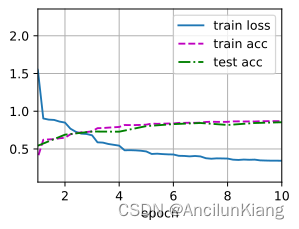
lr, num_epochs = 0.9, 10
train_ch6(net, train_iter, test_iter, num_epochs, lr, d2l.try_gpu())
1
2

loss 0.471, train acc 0.820, test acc 0.815
40056.7 examples/sec on cuda:0
1
2

练习

（1）将平均汇聚层替换为最大汇聚层，会发生什么？

net_Max = nn.Sequential(
    nn.Conv2d(1, 6, kernel_size=5, padding=2), nn.Sigmoid(),
    nn.MaxPool2d(kernel_size=2, stride=2),
    nn.Conv2d(6, 16, kernel_size=5), nn.Sigmoid(),
    nn.MaxPool2d(kernel_size=2, stride=2),
    nn.Flatten(),
    nn.Linear(16 * 5 * 5, 120), nn.Sigmoid(),
    nn.Linear(120, 84), nn.Sigmoid(),
    nn.Linear(84, 10))

lr, num_epochs = 0.9, 10
train_ch6(net_Max, train_iter, test_iter, num_epochs, lr, d2l.try_gpu())
1
2
3
4
5
6
7
8
9
10
11
12

loss 0.422, train acc 0.844, test acc 0.671
31151.6 examples/sec on cuda:0
1
2

几乎无区别

---

（2）尝试构建一个基于 LeNet 的更复杂网络，以提高其精准性。

a. 调节卷积窗口的大小。
b. 调整输出通道的数量。
c. 调整激活函数（如 ReLU）。
d. 调整卷积层的数量。
e. 调整全连接层的数量。
f. 调整学习率和其他训练细节（例如，初始化和轮数）。
1
2
3
4
5
6

net_Best = nn.Sequential(
    nn.Conv2d(1, 8, kernel_size=5, padding=2), nn.ReLU(),
    nn.AvgPool2d(kernel_size=2, stride=2),
    nn.Conv2d(8, 16, kernel_size=3, padding=1), nn.ReLU(),
    nn.AvgPool2d(kernel_size=2, stride=2),
    nn.Conv2d(16, 32, kernel_size=3, padding=1), nn.ReLU(),
    nn.AvgPool2d(kernel_size=2, stride=2),
    nn.Flatten(),
    nn.Linear(32 * 3 * 3, 128), nn.ReLU(),
    nn.Linear(128, 64), nn.ReLU(),
    nn.Linear(64, 32), nn.ReLU(),
    nn.Linear(32, 10)
)
1
2
3
4
5
6
7
8
9
10
11
12
13

lr, num_epochs = 0.4, 10
train_ch6(net_Best, train_iter, test_iter, num_epochs, lr, d2l.try_gpu())
1
2

loss 0.344, train acc 0.869, test acc 0.854
32868.3 examples/sec on cuda:0
1
2

---

（3）在 MNIST 数据集上尝试以上改进后的网络。

import torchvision
from torch.utils import data
from torchvision import transforms

trans = transforms.ToTensor()
mnist_train = torchvision.datasets.MNIST(
    root="../data", train=True, transform=trans, download=True)
mnist_test = torchvision.datasets.MNIST(
    root="../data", train=False, transform=trans, download=True)
train_iter2 = data.DataLoader(mnist_train, batch_size, shuffle=True,
                             num_workers=d2l.get_dataloader_workers())
test_iter2 = data.DataLoader(mnist_test, batch_size, shuffle=True,
                            num_workers=d2l.get_dataloader_workers())

lr, num_epochs = 0.4, 5  # 大约 6 轮往后直接就爆炸
train_ch6(net_Best, train_iter2, test_iter2, num_epochs, lr, d2l.try_gpu())
1
2
3
4
5
6
7
8
9
10
11
12
13
14
15
16

loss 0.049, train acc 0.985, test acc 0.986
26531.1 examples/sec on cuda:0
1
2

---

（4）显示不同输入（例如，毛衣和外套）时 LetNet 第一层和第二层的激活值。

for X, y in test_iter:
        break

x_first_Sigmoid_layer = net[0:2](X)[0:9, 1, :, :]
d2l.show_images(x_first_Sigmoid_layer.reshape(9, 28, 28).cpu().detach(), 1, 9)
x_second_Sigmoid_layer = net[0:5](X)[0:9, 1, :, :]
d2l.show_images(x_second_Sigmoid_layer.reshape(9, 10, 10).cpu().detach(), 1, 9)
d2l.plt.show()
1
2
3
4
5
6
7
8

​

​