【CS324】LLM（大模型的能力、数据、架构、分布式训练、微调等）

note

• 本文是斯坦福大学CS324课程的学习笔记，同时参考了一些LLM相关资料

一、引言

• 语言模型最初是在信息理论的背景下研究的，可以用来估计英语的熵。
  • 熵用于度量概率分布：$$H(p)=\sum _{x}p(x)\log \frac{1}{p(x)}.$$
  • 熵实际上是一个衡量将样本$x\sim p$ 编码（即压缩）成比特串所需要的预期比特数的度量。举例来说，“the mouse ate the cheese” 可能会被编码成 “0001110101”。熵的值越小，表明序列的结构性越强，编码的长度就越短。直观地理解，$\log \frac{1}{p(x)}$ 可以视为用于表示出现概率为$p(x)$的元素$x$的编码的长度。
  • 交叉熵H(p,q)上界是熵H§：$$H(p,q)=\sum _{x}p(x)\log \frac{1}{q(x)}.$$，所以可以通过构建一个只有来自真实数据分布$p$的样本的（语言）模型$q$来估计$H(p,q)$
• N-gram模型在计算上极其高效，但在统计上效率低下。
• 神经语言模型在统计上是高效的，但在计算上是低效的。
• 大模型的参数发展：随着深度学习在2010年代的兴起和主要硬件的进步（例如GPU），神经语言模型的规模已经大幅增加。以下表格显示，在过去4年中，模型的大小增加了5000倍。

二、大模型的能力

1. 从语言模型到任务模型

• 创建一个新模型并利用语言模型作为特征（探针法）
• 模型微调

2. 任务评估

• Language modeling
  • 困惑度：每个标记（token）的平均"分支因子（branching factor）“。这里的"分支因子”，可以理解为在每个特定的词或标记出现后，语言模型预测下一个可能出现的词或标记的平均数量。因此，它实际上是度量模型预测的多样性和不确定性的一种方式。
  • 两类错误：
    • 召回错误
    • 精确度错误
• Question answering：问答
• Translation：翻译
• Arithmetic：抽象推理，如做数学题
• News article generation：给定标题，生成文章
• Novel tasks：给定自定义词语，生成使用该词的句子

相关benchmark：

• SWORDS：词汇替换，目标是在句子的上下文中预测同义词。
• Massive Multitask Language Understanding：包括数学，美国历史，计算机科学等57个多选问题。
• TruthfulQA：人类由于误解而错误回答的问答数据集。

三、大模型的有害性

有害性（上）

• 性能差异：自动语音识别（ASR）系统在黑人说话者的识别性能要差于白人说话者（Koenecke等人，2020）
• 社会偏见：性别歧视等

有害性（下）

• 有毒性：toxicity，如粗鲁、不尊重或不合理的行为，可能使某人想要离开一场对话。如“跨性别女性不是女性”。
• 假信息：disinformation
• 内容审查：Facebook（或Meta）长期以来一直在打击有害内容，最近开始利用语言模型自动检测这类内容。例如，RoBERTa已经被使用了几年。

四、大模型的数据

• Common Crawl是一个非营利组织，它对网络进行爬取，并提供免费给公众的快照。由于其便利性，它已经成为许多模型如T5、GPT-3和Gopher的标准数据源。
  • 网络数据虽然丰富，但是有偏见，比如年轻、男性、用户较多，维基百科只有8.8%的女性编写者等
• 尽管OpenAI并没有公开发布WebText数据集，但OpenWebText数据集在理念上复制了WebText的构建方法。
• GPT-3的数据集主要源自Common Crawl，而Common Crawl又类似于一个参考数据集——WebText。GPT-3下载了41个分片的Common Crawl数据（2016-2019年）。通过训练一个二元分类器来预测WebText与Common Crawl的区别，如果分类器认为文档更接近WebText，那么这个文档就有更大的概率被保留。在处理数据时，GPT-3采用了模糊去重的方法（检测13-gram重叠，如果在少于10个训练文档中出现，则移除窗口或文档），并从基准数据集中移除了数据。此外，GPT-3也扩大了数据来源的多样性（包括WebText2、Books1、Books2以及维基百科）。在训练过程中，Common Crawl被降采样，它在数据集中占82%，但只贡献了60%的数据。
• 大模型pretrain用到的语料：

• 综述《A Survey of Large Language Models》总结的主流大模型的pretrain语料的各部分占比：
  
• 典型的pretrain数据预处理pipeline：异常词过滤、去重、隐私信息处理、tokenization等：

五、law问题

• law问题：
  • 数据：如数据隐私问题
  • 模型应用：用于下游任务，不能做坏事（如欺诈、假新闻、诈骗等）
  • 版权问题
• 信息技术的三大阶段：
  • 1. 第一阶段：文本数据挖掘（搜索引擎），基于简单的模式匹配。
  • 2. 第二阶段：分类（例如，分类停止标志或情感分析），推荐系统。
  • 3. 第三阶段：学习模仿表达的生成模型。

六、模型架构篇

1. tokenization

好的分词：

• 分词后的token不能太多，否则难建模；token也不能太少，否则单词之间无法共享参数
• 每个token标记是一个语言或统计上有意义的单位

分词方法：

• 基于空格的分词：text.split(' ')，最简单的方法，如果是英文是可行，但是中文词语之间没有空格，即使在英语，也有连字符词（例如father-in-law）和缩略词（例如don’t），它们需要被正确拆分。例如，Penn Treebank将don’t拆分为do和n’t，这是一个在语言上基于信息的选择，但不太明显。因此，仅仅通过空格来划分单词会带来很多问题。
• 其他方法：
  • Byte-Pair Encoding (BPE) tokenization
  • WordPiece tokenization
  • Unigram tokenization
  • 可以使用库：SentencePiece
  • 常见的模型使用的tokenizer如下图：

【栗子】
假设我们有一个英文语料库，其中包含以下两个句子：

1. “I like playing soccer.”
2. “I like playing basketball.”

现在，我们想要使用这些句子来构建一个子词词表，以便进行分词。

BPE（Byte Pair Encoding）：

使用 BPE 进行分词时，我们首先将每个句子划分为单个字符，得到以下字符序列：

1. “I like playing soccer.”

   • Characters: [‘I’, ’ ', ‘l’, ‘i’, ‘k’, ‘e’, ’ ', ‘p’, ‘l’, ‘a’, ‘y’, ‘i’, ‘n’, ‘g’, ’ ', ‘s’, ‘o’, ‘c’, ‘c’, ‘e’, ‘r’, ‘.’]

2. “I like playing basketball.”

   • Characters: [‘I’, ’ ', ‘l’, ‘i’, ‘k’, ‘e’, ’ ', ‘p’, ‘l’, ‘a’, ‘y’, ‘i’, ‘n’, ‘g’, ’ ', ‘b’, ‘a’, ‘s’, ‘k’, ‘e’, ‘t’, ‘b’, ‘a’, ‘l’, ‘l’, ‘.’]

然后，我们计算字符序列中最频繁出现的字符组合，并将其合并为一个新的子词。在这个例子中，“pl” 是最频繁出现的字符组合，我们将其合并为一个新的子词，得到以下序列：

1. “I like playing soccer.”

   • Tokens: [‘I’, ’ ', ‘like’, ’ ', ‘playing’, ’ ', ‘s’, ‘o’, ‘c’, ‘e’, ‘r’, ‘.’]

2. “I like playing basketball.”

   • Tokens: [‘I’, ’ ', ‘like’, ’ ', ‘playing’, ’ ', ‘b’, ‘a’, ‘s’, ‘k’, ‘e’, ‘t’, ‘b’, ‘a’, ‘l’, ‘l’, ‘.’]

通过 BPE，我们将 “pl” 作为一个子词，成功地将 “playing” 分割为 “play” 和 “ing”。

WordPiece：

对于 WordPiece 分词，我们也首先将每个句子划分为单个字符。然后，我们根据字符序列的频率和语言模型得分来选择合并操作。

对于上述例子，我们计算字符序列的频率，并选择最频繁出现的合并操作。假设我们选择合并 “pl”：

1. “I like playing soccer.”

   • Tokens: [‘I’, ’ ', ‘like’, ’ ', ‘p’, ‘lay’, ‘ing’, ’ ', ‘soccer’, ‘.’]

2. “I like playing basketball.”

   • Tokens: [‘I’, ’ ', ‘like’, ’ ', ‘p’, ‘lay’, ‘ing’, ’ ', ‘basketball’, ‘.’]

通过 WordPiece，我们成功地将 “playing” 分割为 “p”, “lay” 和 “ing”。

总结：

• BPE 和 WordPiece 是基于统计的子词分词方法，可以将频繁出现的字符组合合并为子词。
• BPE 是通过简单的频率统计来合并字符组合，而 WordPiece 还考虑了语言模型得分。

2. 模型架构

上下文向量表征 (Contextual Embedding)举例如下，标记的上下文向量表征取决于其上下文（周围的单词）；例如，考虑mouse的向量表示需要关注到周围某个窗口大小的其他单词：
[ t h e , m o u s e , a t e , t h e , c h e e s e ] ⇒ ϕ [ ( 1 0.1 ) , ( 0 1 ) , ( 1 1 ) , ( 1 − 0.1 ) , ( 0 − 1 ) ] . [the, mouse, ate, the, cheese] \stackrel{\phi}{\Rightarrow}\left[\left(

\right),\left(\right),\left(\right),\left(\right),\left(\right)\right]. [the,mouse,ate,the,cheese]⇒ϕ[(10.1​),(01​),(11​),(1−0.1​),(0−1​)].

• 符号表示：将 $\varphi :V^L\to R^{d\times L}$ 定义为嵌入函数（类似于序列的特征映射，映射为对应的向量表示）。
• 对于标记序列 $x1:L=[x_1,\dots ,x_L]$，$\varphi$ 生成上下文向量表征 $\varphi (x_{1:L})$。

（1）only encoder

• 模型：bert、RoBERTa等，生成上下文向量，而不是直接生成文本，常用于作分类任务
• 优点：对于每个 $xi$，上下文向量表征可以双向地依赖于左侧上下文 $(x_{1:i-1})$ 和右侧上下文 $(x_{i+1:L})$。

（2）only decoder

• 模型：gpt就是自回归模型，给定一个提示 $x_{1:i}$，它们可以生成上下文向量表征，并对下一个标记 $x_{i+1}$（以及递归地，整个完成 $x_{i+1:L}$）生成一个概率分布。$x_{1:i}\Rightarrow \varphi (x_{1:i}),p(x_{i+1}\mid x_{1:i})$。
• 缺点：对于每个 $xi$，上下文向量表征只能单向地依赖于左侧上下文 ($x_{1:i-1}$)。

（3）encoder-decoder

• 模型：最初的transformer、BART、T5等
• 优点：它们可以使用双向上下文向量表征来处理输入 $x_{1:L}$，并且可以生成输出 $y_{1:L}$。可以公式化为：
  $$x1:L\Rightarrow \varphi (x1:L),p(y1:L\mid \varphi (x1:L))。$$
  以表格到文本生成任务为例，其输入和输出的可以表示为：
  $$[名称:,植物,|,类型:,花卉,商店]\Rightarrow [花卉,是,一,个,商店]。$$
• 缺点：需要更多的特定训练目标

3. 基础架构

（1）回归transformer架构

单头注意力矩阵形式：
def $Attention(x_{1:L}:R^{d\times L},y:R^d)\to R^d$：

• 通过将其与每个$x_i$进行比较来处理$y$。
• 返回$W_{value}{x}_{1:L}\mathrm{softmax}\left(x_{1:L}^{\top }{W}_{key}^{\top }{W}_{query}y/\sqrt{d}\right)$

多头注意力机制：
def $MultiHeadedAttention(x_{1:L}:R^{d\times L},y:R^d)\to R^d$:

• 通过将其与每个xi与nheads个方面进行比较，处理y。
• 返回$W_{output}[\underset{n_{heads}times}{\underbrace{\left[\mathrm{Attention}\left(x_{1:L},y\right),\dots ,\mathrm{Attention}\left(x_{1:L},y\right)\right]}}$

对于自注意层，我们将用$x_i$替换$y$作为查询参数来产生，其本质上就是将自身的$x_i$对句子的其他上下文内容进行$Attention$的运算：

def $SelfAttention(x_{1:L}:R_{d\times L})\to R_{d\times L})$：

• 将每个元素xi与其他元素进行比较。
• 返回$[Attention(x_{1:L},x_1),\dots ,Attention(x_{1:L},x_L)]$。

自注意力使得所有的标记都可以“相互通信”，而前馈层提供进一步的连接：

def $FeedForward(x_{1:L}:R^{d\times L})\to R^{d\times L}$：

• 独立处理每个标记。
• 对于$i=1,\dots ,L$：
  • 计算$y_i=W_{2}max(W_1{x}_i+b_1,0)+b_2$。
• 返回$[y_1,\dots ,y_L]$。
  

（2）优化网络训练

（1）残差链接：添加残差（跳跃）连接，防止$f$梯度消失时还可以使用$x_{1:L}$计算
（2）层归一化：def $LayerNorm(x_{1:L}:R^{d\times L})\to R^{d\times L}$，具体而言定义函数接受一个序列模型$f$并使其“鲁棒”：

def $AddNorm(f:(R{d}^{\times L}\to R^{d\times L}),x_{1:L}:R_{d\times L})\to R^{d\times L}$：

• 将f应用于$x_{1:L}$。
• 返回$LayerNorm(x_{1:L}+f(x_{1:L}))$。

最后定义Transformer块如下：

def $TransformerBlock(x_{1:L}:R^{d\times L})\to R^{d\times L}$：

• 处理上下文中的每个元素$x_i$。
• 返回$AddNorm(FeedForward,AddNorm(SelfAttention,x_{1:L}))$。

（3）位置嵌入
def $EmbedTokenWithPosition(x_{1:L}:R^{d\times L})$：

• 添加位置信息。
• 定义位置嵌入：
  • 偶数维度：$P_{i,2j}=sin(i/10000^{2j/dmodel})$
  • 奇数维度：$P_{i,2j+1}=cos(i/10000^{2j/dmodel})$
• 返回$[x_1+P_1,\dots ,x_L+P_L]$。
• 上面的标记：$i$表示句子中标记的位置，$j$表示该标记的向量表示维度位置。

注意：现在LLM大模型还有使用ROPE旋转位置编码、ALiBi位置编码等扩大窗口大小。

4. 大模型架构

（1）GPT3架构：

• 将transformer块堆叠96次
• 隐藏状态的维度：dmodel=12288
• 中间前馈层的维度：dff=4dmodel
• 注意头的数量：nheads=96
• 上下文长度：L=2048

（2）llama模型架构

• transformer architecture (Vaswani et al., 2017),
• 使用RMSNorm(Root Mean Square Layer Normalization)方法对transformer每层的输入进行归约(norm)操作，代替了transformer之前对输出进行归约(norm)：apply pre-normalization using RMSNorm (Zhang and Sennrich, 2019),
• SwiGLU激活函数：use the SwiGLU activation function (Shazeer, 2020),
• 旋转位置编码：rotary positional embeddings(RoPE, Su et al. 2022).
• 上下文长度和分组查询注意力(GQA)：The primary architectural differences from Llama 1 include increased context length and grouped-query attention (GQA).

七、模型训练

1. decoder-only模型

自回归语言模型的条件分布$p(x_i\mid x_{1:i-1})$：

• 将$x_{1:i-1}$映射到上下文嵌入$\varphi (x_{1:i-1})$。
• 应用嵌入矩阵$E\in {\mathbb{R}}^{V\times d}$来获得每个token的得分$E\varphi (x_{1:i-1}{)}_{i-1}$。
• 对其进行指数化和归一化，得到预测$x_i$的分布。
• 总结为：
  $$p(x_{i+1}\mid x_{1:i})=softmax(E\varphi (x_{1:i}{)}_i).$$

最大似然：设$\theta$是大语言模型的所有参数。设$D$是由一组序列组成的训练数据。然后可以遵循最大似然原理，定义以下负对数似然目标函数：
$$O(\theta )=\sum _{x\in D}-\log p_{\theta }(x)=\sum _{x\in D}\sum _{i=1}^L-\log p_{\theta }(x_i\mid x_{1:i-1}).$$

2. 优化算法

已知：自回归语言模型的目标函数：$$O(\theta )=\sum _{x\in D}-\log p_{\theta }(x).$$

（1）Adam (adaptive moment estimation)

Adam算法拥有以下两个创新：

1. 引入动量（继续朝同一方向移动）。
2. 参数${\theta }_0$的每个维度都有一个自适应（不同）的步长（受二阶方法启发）。

它的步骤如下：

• 初始化参数${\theta }_0$

• 初始化动量$m_0,v_0\leftarrow 0$

• 重复以下步骤：

  • 采样小批量$B_t\subset D$

  • 按照如下步骤更新参数：

    • 计算梯度

    $$g_t\leftarrow \frac{1}{|B_t|}\sum _{x\in B_t}{\nabla }_{\theta }(-\log p_{\theta }(x)).$$

    • 更新一阶、二阶动量

    $$\begin{gathered} m_t\leftarrow {\beta }_1{m}_{t-1}+(1-{\beta }_1)g_t \\ {v}_t\leftarrow {\beta }_2{v}_{t-1}+(1-{\beta }_2)g_t^2 \end{gathered}$$

    • 对偏差进行修正

    $$\begin{gathered} {\hat{m}}_t\leftarrow m_t/(1-{\beta }_1^t) \\ {\hat{v}}_t\leftarrow v_t/(1-{\beta }_2^t) \end{gathered}$$

    • 更新参数

    $${\theta }_t\leftarrow {\theta }_{t-1}-\eta {\hat{m}}_t/(\sqrt{{\hat{v}}_t}+ϵ).$$

存储占用分析：

Adam将存储从2倍的模型参数（${\theta }_t,g_t$）增加到了4倍（${\theta }_t,g_t,m_t,v_t$）。

（2） AdaFactor

AdaFactor是一种为减少存储占用的优化算法。特点：

• 它不储存$m_t,v_t$这样的$O(m\times n)$矩阵，而是存储行和列的和$O(m+n)$并重构矩阵
• 去除动量
• 它被用来训练T5
• AdaFactor可能使训练变得困难（见Twitter thread和blog post）

（3）模型参数初始化

• 给定矩阵$W\in {\mathbb{R}}^{m\times n}$，标准初始化（即，xavier初始化）为$W_{ij}\sim N(0,1/n)$。
• GPT-2和GPT-3通过额外的$1/\sqrt{N}$缩放权重，其中$N$是残差层的数量。
• T5将注意力矩阵增加一个$1/\sqrt{d}（$代码）。

以GPT-3为例，使用的参数如下：

• Adam参数：${\beta }_1=0.9,{\beta }_2=0.95,ϵ=10^{-8}$
• 批量小：320万个token（约1500个序列）
• 使用梯度剪裁（$g_t\leftarrow g_t/\min (1,\Vert g{\Vert }_2)$）
• 线性学习率预热（前3.75亿个token）
• 余弦学习率衰减到10%
• 逐渐增加批大小
• 权重衰减设为0.1

八、分布式训练

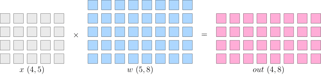
【背景】假设神经网络中某一层是做矩阵乘法, 其中的输入 $x$ 的形状为 $4\times 5$, 模型参数 $w$ 的形状为 $5\times 8$, 那么, 矩阵乘法输出形状为 $4\times 8$ 。如下:

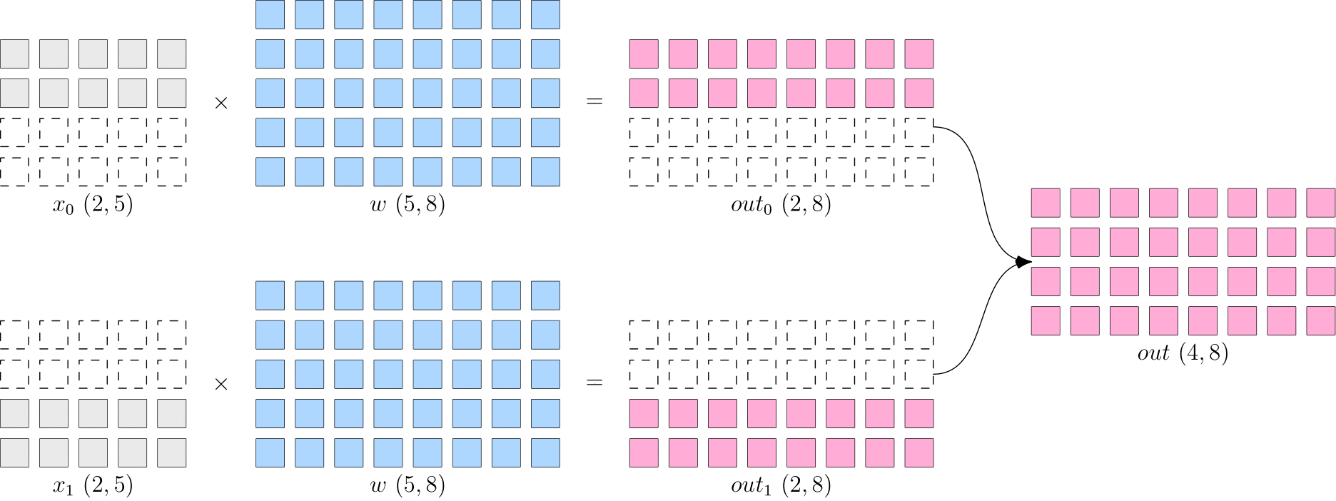
• 数据并行：切分数据$x$到不同设备上，在反向传播过程中，需要对各个设备上的梯度进行 AllReduce，以确保各个设备上的模型始终保持一致。适合数据较大，模型较小的情况，如resnet50

  • allReduce： 先将所有device上的模型的梯度reduce归约，然后将结果广播到所有设备上
    

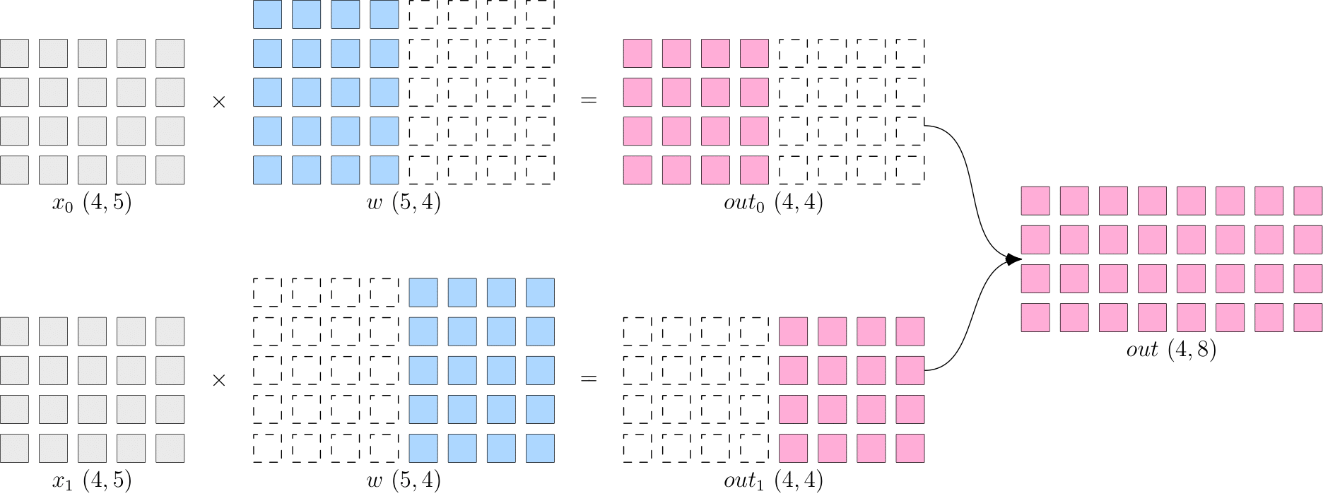
• 模型并行：省去了多个设备之间的梯度 AllReduce；但是, 由于每个设备都需要完整的数据输入，因此，数据会在多个设备之间进行广播，产生通信代价。比如，上图中的最终得到的 out $(4\times 8)$ ，如果它作为下一层网络的输入，那么它就需要被广播发送到两个设备上。如bert
  

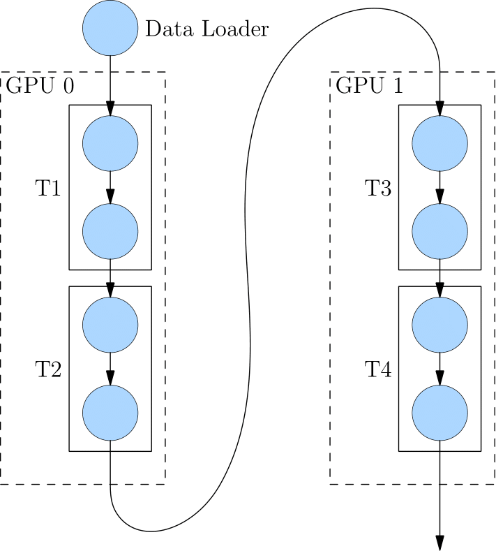
• 流水并行：模型网络过大，除了用模型并行，还能用流水并行（如下的网络有4层，T1-T4）
  

• 混合并行：综合上面的多种策略一起训练，如GPT3：

  • 首先被分为 64 个阶段，进行流水并行。每个阶段都运行在 6 台 DGX-A100 主机上。
  • 在6台主机之间，进行的是数据并行训练；
  • 每台主机有 8 张 GPU 显卡，同一台机器上的8张 GPU 显卡之间是进行模型并行训练。

参考：

• stanford course：https://stanford-cs324.github.io/winter2022/lectures/parallelism/
• Megatron-LM: Training Multi-Billion Parameter Language Models Using Model Parallelism. M. Shoeybi, M. Patwary, Raul Puri, P. LeGresley, J. Casper, Bryan Catanzaro. 2019.
• GPipe: Efficient Training of Giant Neural Networks using Pipeline Parallelism. Yanping Huang, Yonglong Cheng, Dehao Chen, HyoukJoong Lee, Jiquan Ngiam, Quoc V. Le, Z. Chen. NeurIPS 2018.
• Efficient large-scale language model training on GPU clusters using Megatron-LM. D. Narayanan, M. Shoeybi, J. Casper, P. LeGresley, M. Patwary, V. Korthikanti, Dmitri Vainbrand, Prethvi Kashinkunti, J.Bernauer, Bryan Catanzaro, Amar Phanishayee, M. Zaharia. SC 2021.
• TeraPipe: Token-Level Pipeline Parallelism for Training Large-Scale Language Models. Zhuohan Li, Siyuan Zhuang, Shiyuan Guo, Danyang Zhuo, Hao Zhang, D. Song, I. Stoica. ICML 2021.

九、新的模型架构

• 混合专家模型有点以前MMOE的味道，基于检索的模型可以和知识库问答结合，具体模型后期再研究更新，读者大佬们多催催我谢谢。

1. 混合专家模型

参考资料：

• Outrageously Large Neural Networks: The Sparsely-Gated Mixture-of-Experts Layer. Noam M. Shazeer, Azalia Mirhoseini, Krzysztof Maziarz, Andy Davis, Quoc V. Le, Geoffrey E. Hinton, J. Dean. ICLR 2017. Trains 137 billion parameter model; mixture of experts (1000 experts) applied convolutionally between LSTM layers.
• GShard: Scaling Giant Models with Conditional Computation and Automatic Sharding. Dmitry Lepikhin, HyoukJoong Lee, Yuanzhong Xu, Dehao Chen, Orhan Firat, Yanping Huang, M. Krikun, Noam M. Shazeer, Z. Chen. ICLR 2020. Trains Transformer for neural machine translation (100 languages) with 600 billion parameters. Use top-2 experts.
• Switch Transformers: Scaling to Trillion Parameter Models with Simple and Efficient Sparsity. W. Fedus, Barret Zoph, Noam M. Shazeer. 2021. Trains language model, 4x speedup over T5-XXL (13 billion parameters). Use top-1 expert.
• GLaM: Efficient Scaling of Language Models with Mixture-of-Experts. Nan Du, Yanping Huang, Andrew M. Dai, Simon Tong, Dmitry Lepikhin, Yuanzhong Xu, M. Krikun, Yanqi Zhou, Adams Wei Yu, Orhan Firat, Barret Zoph, Liam Fedus, Maarten Bosma, Zongwei Zhou, Tao Wang, Yu Emma Wang, Kellie Webster, Marie Pellat, Kevin Robinson, K. Meier-Hellstern, Toju Duke, Lucas Dixon, Kun Zhang, Quoc V. Le, Yonghui Wu, Zhifeng Chen, Claire Cui. 2021. Trains 1.2 trillion parameter model, 64 experts. Use top-2 experts. Also creates new dataset.
• BASE Layers: Simplifying Training of Large, Sparse Models. M. Lewis, Shruti Bhosale, Tim Dettmers, Naman Goyal, Luke Zettlemoyer. ICML 2021. Solve optimization problem for token-to-expert allocation to balance allocation. Trains 110 billion parameter model.
• Efficient Large Scale Language Modeling with Mixtures of Experts. Mikel Artetxe, Shruti Bhosale, Naman Goyal, Todor Mihaylov, Myle Ott, Sam Shleifer, Xi Victoria Lin, Jingfei Du, Srinivasan Iyer, Ramakanth Pasunuru, Giridhar Anantharaman, Xian Li, Shuohui Chen, H. Akın, Mandeep Baines, Louis Martin, Xing Zhou, Punit Singh Koura, Brian O’Horo, Jeff Wang, Luke Zettlemoyer, Mona Diab, Zornitsa Kozareva, Ves Stoyanov. 2021. Trains 1.1 trillion parameter models. Use top-2 experts (512 experts).
• Towards Crowdsourced Training of Large Neural Networks using Decentralized Mixture-of-Experts. Max Ryabinin, Anton I. Gusev. NeurIPS 2020.
• Distributed Deep Learning in Open Collaborations. Michael Diskin, Alexey Bukhtiyarov, Max Ryabinin, Lucile Saulnier, Quentin Lhoest, A. Sinitsin, Dmitry Popov, Dmitry Pyrkin, M. Kashirin, Alexander Borzunov, Albert Villanova del Moral, Denis Mazur, Ilia Kobelev, Yacine Jernite, Thomas Wolf, Gennady Pekhimenko. 2021.
• Dense-to-Sparse Gate for Mixture-of-Experts. Xiaonan Nie, Shijie Cao, Xupeng Miao, Lingxiao Ma, Jilong Xue, Youshan Miao, Zichao Yang, Zhi Yang, Bin Cui. 2021.

2. 基于检索的模型

参考资料：

• REALM: Retrieval-Augmented Language Model Pre-Training. Kelvin Guu, Kenton Lee, Z. Tung, Panupong Pasupat, Ming-Wei Chang. 2020. Introduces REALM.
• Retrieval-Augmented Generation for Knowledge-Intensive NLP Tasks. Patrick Lewis, Ethan Perez, Aleksandara Piktus, Fabio Petroni, Vladimir Karpukhin, Naman Goyal, Heinrich Kuttler, M. Lewis, Wen-tau Yih, Tim Rocktäschel, Sebastian Riedel, Douwe Kiela. NeurIPS 2020. Introduces RAG.
• Improving language models by retrieving from trillions of tokens. Sebastian Borgeaud, A. Mensch, Jordan Hoffmann, Trevor Cai, Eliza Rutherford, Katie Millican, G. V. D. Driessche, J. Lespiau, Bogdan Damoc, Aidan Clark, Diego de Las Casas, Aurelia Guy, Jacob Menick, Roman Ring, T. Hennigan, Saffron Huang, Lorenzo Maggiore, Chris Jones, Albin Cassirer, Andy Brock, Michela Paganini, Geoffrey Irving, Oriol Vinyals, Simon Osindero, K. Simonyan, Jack W. Rae, Erich Elsen, L. Sifre. 2021. Introduces RETRO.

十、大模型的adaption

1. 通用的adaptation配置

1. 预训练语言模型（Pre-trained LM）:
   用参数$\theta LM$表示

2. 下游任务数据集（Downstream Task Dataset）:
   下游任务分布$P_{task}$的样本数据。可以是文本分类、情感分析等任务的特定实例，每个样本由输入x和目标输出y组成，如：$\left(x^{(1)},y^{(1)}\right),\dots ,\left(x^{(n)},y^{(n)}\right)$。

3. 适配参数（Adaptation Parameters）:
   为了使预训练的LM适合特定的下游任务，现在需要找到一组参数$\gamma$，这组参数可以来自现有参数的子集或引入的新的参数，$\Gamma$。这些参数将用于调整模型，以便它在特定任务上的表现更好。

4. 任务损失函数（Task Loss Function）:
   定义一个损失函数${\ell }_{\text{task }}$来衡量模型在下游任务上的表现。例如，交叉熵损失是一种常见的选择，用于衡量模型预测的概率分布与真实分布之间的差异。

5. 优化问题（Optimization Problem）:
   目标是找到一组适配参数${\gamma }_{\text{adapt }}$，使得任务损失在整个下游数据集上最小化。数学上，这可以通过以下优化问题表示：

$${\gamma }_{\text{adapt }}={\mathrm{argmin}}_{\gamma \in \Gamma }\frac{1}{n}\sum _{i=1}^n{\ell }_{\text{task }}\left(\gamma ,{\theta }_{\mathrm{LM}},x_i,y_i\right).$$
最后取得一组适配参数${\gamma }_{\text{adapt }}$，用于参数化适配后的模型$p_{adapt}$。

2. Adaptation方法

（1）Probing

（2）Fine-tuning

人类对齐的fine-tuning

InstructGPT对GPT-3模型进行微调的三个步骤：

1. 收集人类书写的示范行为：这一步骤涉及收集符合人类期望的示例，并对这些示例进行监督微调。

2. 基于指令的采样与人类偏好：对于每个指令，从步骤1的LM中采样k个输出。然后收集人类对哪个采样输出最优先的反馈。与步骤1相比，这些数据更便宜。

3. 使用强化学习目标微调LM：通过强化学习目标微调步骤1中的LM，以最大化人类偏好奖励。

经过这样的微调，1.3B的InstructGPT模型在85%的时间里被优先于175B的GPT-3，使用少样本提示时为71%。在封闭领域的问答/摘要方面，InstructGPT 21%的时间会产生虚构信息，相比GPT-3的41%有所改善。在被提示要尊重时，InstructGPT比GPT-3减少了25%的有毒输出。

（3）Lightweight Fine-tuning

• 可以借助peft库（Parameter-Efficient Fine-Tuning）进行微调，支持如下tuning：
  • Adapter Tuning（固定原预训练模型的参数 只对新增的adapter进行微调）
  • Prefix Tuning（在输入token前构造一段任务相关的virtual tokens作为prefix，训练时只更新Prefix部分的参数，而Transformer的其他不分参数固定，和构造prompt类似，只是prompt是人为构造的即无法在模型训练时更新参数，而Prefix可以学习<隐式>的prompt）
  • Prompt Tuning（Prefix Tuning的简化版，只在输入层加入prompt tokens，并不需要加入MLP）
  • P-tuning（将prompt转为可学习的embedding层，v2则加入了prompts tokens作为输入）
  • LoRA（Low-Rank Adaption，为了解决adapter增加模型深度而增加模型推理时间、上面几种tuning中prompt较难训练，减少模型的可用序列长度）
    • 该方法可以在推理时直接用训练好的AB两个矩阵和原预训练模型的参数相加，相加结果替换原预训练模型参数。
    • 相当于用LoRA模拟full-tunetune过程

Lightweight Fine-tuning节省资源的同时保持和全参微调相同的效果：

1. 提示调整（Prompt Tuning）：通过微调模型的输入prompt提示来优化模型的表现。提示调整可以被视为一种更灵活的微调方法，允许用户通过调整输入提示来导向模型的输出，而不是直接修改模型参数。
2. 前缀调整（Prefix Tuning）：与提示调整类似，前缀调整也集中在输入部分。它通过添加特定前缀来调整模型的行为，从而对特定任务进行定制。
3. 适配器调整（Adapter Tuning）：适配器调整是通过在模型的隐藏层之间插入可训练的“适配器”模块来微调模型的一种方法。这些适配器模块允许模型在不改变原始预训练参数的情况下进行微调，从而降低了存储和计算的需求。

十一、环境影响

Patterson et al., 2021
简单形式：
$$\text{emissions}=R_{\text{power}\to \text{emit}}(\text{energy-train}+\text{queries}\cdot \text{energy-inference})$$

• NVIDIA：80%的ML工作负载是推理，而不是训练

对于训练：

$$\text{emissions}=\text{hours-to-train}\cdot \text{num-processors}\cdot \text{power-per-processor}\cdot \text{PUE}\cdot R_{\text{power}\to \text{emit}}$$

不同模型的估计值：

• T5：86 MWh，47t CO2eq
• GShard（用于机器翻译的MOE模型）：24 MWh，4.3t CO2eq
• Switch Transformer：179 MWh，59t CO2eq
• GPT3：1287 MWh，552t CO2eq

Reference

[1] 斯坦福大学CS324课程：https://stanford-cs324.github.io/winter2022/lectures/introduction/#a-brief-history
[2] CS224N lecture notes on language models
[3] Language Models are Few-Shot Learners. Tom B. Brown, Benjamin Mann, Nick Ryder, Melanie Subbiah, J. Kaplan, Prafulla Dhariwal, Arvind Neelakantan, Pranav Shyam, Girish Sastry, Amanda Askell, Sandhini Agarwal, Ariel Herbert-Voss, Gretchen Krueger, T. Henighan, R. Child, A. Ramesh, Daniel M. Ziegler, Jeff Wu, Clemens Winter, Christopher Hesse, Mark Chen, Eric Sigler, Mateusz Litwin, Scott Gray, Benjamin Chess, Jack Clark, Christopher Berner, Sam McCandlish, Alec Radford, Ilya Sutskever, Dario Amodei. NeurIPS 2020.
[4] Challenges in Detoxifying Language Models. Johannes Welbl, Amelia Glaese, Jonathan Uesato, Sumanth Dathathri, John F. J. Mellor, Lisa Anne Hendricks, Kirsty Anderson, P. Kohli, Ben Coppin, Po-Sen Huang. EMNLP 2021.
[5] Scaling Language Models: Methods, Analysis&Insights from Training Gopher
[5] CommonCrawl
[6] OpenWebText Similar to WebText, used to train GPT-2.
[7] An Empirical Exploration in Quality Filtering of Text Data. Leo Gao. 2021.
[8] Deduplicating Training Data Makes Language Models Better. Katherine Lee, Daphne Ippolito, Andrew Nystrom, Chiyuan Zhang, D. Eck, Chris Callison-Burch, Nicholas Carlini. 2021.
[9] Foundation models report (legality section)
[10] A Survey of Large Language Models：http://arxiv.org/abs/2303.18223
[11] Attention is All you Need. Ashish Vaswani, Noam M. Shazeer, Niki Parmar, Jakob Uszkoreit, Llion Jones, Aidan N. Gomez, Lukasz Kaiser, Illia Polosukhin. NIPS 2017.
[12] CS224N slides on Transformers
[13] Rethinking Attention with Performers. K. Choromanski, Valerii Likhosherstov, David Dohan, Xingyou Song, Andreea Gane, Tamás Sarlós, Peter Hawkins, Jared Davis, Afroz Mohiuddin, Lukasz Kaiser, David Belanger, Lucy J. Colwell, Adrian Weller. ICLR 2020. Introduces Performers.
[14] Efficient Transformers: A Survey. Yi Tay, M. Dehghani, Dara Bahri, Donald Metzler. 2020.
[15] BERT: Pre-training of Deep Bidirectional Transformers for Language Understanding. Jacob Devlin, Ming-Wei Chang, Kenton Lee, Kristina Toutanova. NAACL 2019. Introduces BERT from Google.
[16] RoBERTa: A Robustly Optimized BERT Pretraining Approach. Yinhan Liu, Myle Ott, Naman Goyal, Jingfei Du, Mandar Joshi, Danqi Chen, Omer Levy, M. Lewis, Luke Zettlemoyer, Veselin Stoyanov. 2019. Introduces RoBERTa from Facebook.
[17] BART: Denoising Sequence-to-Sequence Pre-training for Natural Language Generation, Translation, and Comprehension. M. Lewis, Yinhan Liu, Naman Goyal, Marjan Ghazvininejad, Abdelrahman Mohamed, Omer Levy, Veselin Stoyanov, Luke Zettlemoyer. ACL 2019. Introduces BART from Facebook.
[18] Language Models are Few-Shot Learners. Tom B. Brown, Benjamin Mann, Nick Ryder, Melanie Subbiah, J. Kaplan, Prafulla Dhariwal, Arvind Neelakantan, Pranav Shyam, Girish Sastry, Amanda Askell, Sandhini Agarwal, Ariel Herbert-Voss, Gretchen Krueger, T. Henighan, R. Child, A. Ramesh, Daniel M. Ziegler, Jeff Wu, Clemens Winter, Christopher Hesse, Mark Chen, Eric Sigler, Mateusz Litwin, Scott Gray, Benjamin Chess, Jack Clark, Christopher Berner, Sam McCandlish, Alec Radford, Ilya Sutskever, Dario Amodei. NeurIPS 2020. Introduces GPT-3 from OpenAI.
[19] Fixing Weight Decay Regularization in Adam. I. Loshchilov, F. Hutter. 2017. 介绍了AdamW
[20] 混合精度训练
[21] 通俗易懂讲解大模型：Tokenizer
[22] huggingface官方文档解释：Summary of the tokenizers
[23] 微软guidance：https://github.com/guidance-ai/guidance#token-healing-notebook
[24] Understanding Byte-Pair Encoding (BPE) Word Piece And Unigram
[25] 【西湖大学 张岳老师｜自然语言处理在线课程 第十六章 - 4节】BPE（Byte-Pair Encoding）编码
[26] 【LLM系列之Tokenizer】如何科学地训练一个LLM分词器
[27] 大词表语言模型在续写任务上的一个问题及对策. 苏剑林（比如LLM使用超大词表后，“白云”、“白云山”、“白云机场”都是一个独立的token时，用户输入“广州的白云”后，接下来也几乎不会续写出“广州的白云机场”、“广州的白云山”）
[28] 随机分词浅探：从Viterbi Decoding到Viterbi Sampling. 苏剑林
[29] Subword Regularization: Improving Neural Network Translation Models with Multiple Subword Candidates：https://arxiv.org/abs/1804.10959
[30] 常见的分布式并行策略.oneflow

附：时间安排