遥感图像应用：在低分辨率图像上实现洪水损害检测（迁移学习）

本文是上一篇关于“在低分辨率图像上实现洪水损害检测”的博客的延申。

代码来源：https://github.com/weining20000/Flooding-Damage-Detection-from-Post-Hurricane-Satellite-Imagery-Based-on-CNN/tree/master

数据储存地址：https://github.com/JeffereyWu/FloodDamageDetection/tree/main

目标：利用迁移学习训练两个预训练的CNN模型（VGG和Resnet），自动化识别一个区域是否存在洪水损害。

运行环境：Google Colab

1. 导入库

# Pytoch
import torch
from torchvision import datasets, models
from torch.utils.data import Dataset, DataLoader
import torchvision.transforms as transforms
import torch.nn as nn
from torch_lr_finder import LRFinder

# Data science tools
import numpy as np
import pandas as pd
import os
from sklearn.metrics import accuracy_score
from sklearn.metrics import confusion_matrix

from PIL import Image

# Visualizations
import matplotlib.pyplot as plt
import seaborn as sns
1
2
3
4
5
6
7
8
9
10
11
12
13
14
15
16
17
18
19
20

2. 迁移学习知识点

• 对于卷积神经网络（CNN）等模型，通常包括一些卷积层和池化层，这些层的权重用于提取图像的特征。当这些层的参数被冻结时，这些权重将保持不变，不会在训练过程中进行更新。这意味着模型会继续使用预训练模型的特征提取能力。
• 如果模型还包含其他的预训练层，例如预训练的全连接层，这些层的权重也将被冻结，不会更新。
• 通常，当使用预训练模型进行微调时，会替换模型的最后一层或几层，以适应新的任务。新添加的自定义分类器层的权重将被训练和更新，以适应特定的分类任务。

3. 加载和配置预训练的深度学习模型

#Load pre-trained model
def get_pretrained_model(model_name):
  """
  获取预训练模型的函数。

  参数：
  model_name: 要加载的预训练模型的名称（例如，'vgg16' 或 'resnet50'）

  返回：
  MODEL: 加载并配置好的预训练模型
  """

  if model_name == 'vgg16':
      model = models.vgg16(pretrained=True)

      # 将模型的参数（权重）冻结，不进行微调。这意味着这些参数在训练过程中不会更新
      for param in model.parameters():
          param.requires_grad = False
      n_inputs = model.classifier[6].in_features # 获取模型分类器最后一层的输入特征数
      n_classes = 2

      # 替换模型的分类器部分，添加自定义的分类器
      model.classifier[6] = nn.Sequential(
          nn.Linear(n_inputs, 256), nn.ReLU(), nn.Dropout(0.2),
          nn.Linear(256, n_classes))

  elif model_name == 'resnet50':
      model = models.resnet50(pretrained=True)

      for param in model.parameters():
          param.requires_grad = False

	  # 获取模型最后一层全连接层的输入特征数
      n_inputs = model.fc.in_features
      n_classes = 2
      model.fc = nn.Sequential(
          nn.Linear(n_inputs, 256), nn.ReLU(), nn.Dropout(0.2),
          nn.Linear(256, n_classes))

  # Move to GPU
  MODEL = model.to(device)

  return MODEL # 返回加载和配置好的预训练模型
1
2
3
4
5
6
7
8
9
10
11
12
13
14
15
16
17
18
19
20
21
22
23
24
25
26
27
28
29
30
31
32
33
34
35
36
37
38
39
40
41
42
43

注意，这里vgg16的classifier结构原本为：
Sequential(
(0): Linear(in_features=25088, out_features=4096, bias=True)
(1): ReLU(inplace=True)
(2): Dropout(p=0.5, inplace=False)
(3): Linear(in_features=4096, out_features=4096, bias=True)
(4): ReLU(inplace=True)
(5): Dropout(p=0.5, inplace=False)
(6): Linear(in_features=4096, out_features=1000, bias=True)
)
以上代码替换了最后一层的classifier，改为：
Sequential(
(0): Linear(in_features=25088, out_features=4096, bias=True)
(1): ReLU(inplace=True)
(2): Dropout(p=0.5, inplace=False)
(3): Linear(in_features=4096, out_features=4096, bias=True)
(4): ReLU(inplace=True)
(5): Dropout(p=0.5, inplace=False)
(6): Sequential(
(0): Linear(in_features=4096, out_features=256, bias=True)
(1): ReLU()
(2): Dropout(p=0.2, inplace=False)
(3): Linear(in_features=256, out_features=2, bias=True)
)
)

注意，这里resnet50的fc结构原本为：
Linear(in_features=2048, out_features=1000, bias=True)
以上代码替换了最后一层fc，改为：
Sequential(
(0): Linear(in_features=2048, out_features=256, bias=True)
(1): ReLU()
(2): Dropout(p=0.2, inplace=False)
(3): Linear(in_features=256, out_features=2, bias=True)
)

4. 建立模型

# VGG 16
model_vgg = get_pretrained_model('vgg16') # 包含加载和配置好的 VGG16 模型
criterion_vgg = nn.CrossEntropyLoss()
optimizer_vgg = torch.optim.Adam(model_vgg.parameters(), lr=0.00002)

# ResNet 50
model_resnet50 = get_pretrained_model('resnet50') # 包含加载和配置好的 ResNet50 模型
criterion_resnet50 = nn.CrossEntropyLoss() 
optimizer_resnet50 = torch.optim.Adam(model_resnet50.parameters(), lr=0.001)
1
2
3
4
5
6
7
8
9

5. 定义计算准确率的函数

def acc_vgg(x, y, return_labels=False):

  with torch.no_grad(): # 禁止梯度计算，因为在准确率计算中不需要梯度信息
      logits = model_vgg(x)
      pred_labels = np.argmax(logits.cpu().numpy(), axis=1)
  if return_labels:
      return pred_labels
  else:
      return 100*accuracy_score(y.cpu().numpy(), pred_labels)

def acc_resnet50(x, y, return_labels=False):
  
  with torch.no_grad():
      logits = model_resnet50(x)
      pred_labels = np.argmax(logits.cpu().numpy(), axis=1)
  if return_labels:
      return pred_labels
  else:
      return 100*accuracy_score(y.cpu().numpy(), pred_labels)
1
2
3
4
5
6
7
8
9
10
11
12
13
14
15
16
17
18
19

6. 定义一个用于训练深度学习模型的函数

def train(model, criterion, optimizer, acc, xtrain, ytrain, xval, yval, save_file_name, n_epochs, BATCH_SIZE):
    """
    训练深度学习模型的函数。

    参数：
    model: 要训练的深度学习模型
    criterion: 损失函数
    optimizer: 优化器
    acc: 准确率计算函数
    xtrain: 训练数据
    ytrain: 训练标签
    xval: 验证数据
    yval: 验证标签
    save_file_name: 保存训练后模型权重的文件名
    n_epochs: 训练的总轮数（epochs）
    BATCH_SIZE: 每个批次的样本数量

    返回：
    训练完成的模型和训练历史记录
    """

    history1 = []

    # Number of epochs already trained (if using loaded in model weights)
    try:
        print(f'Model has been trained for: {model.epochs} epochs.\n')
    except:
        model.epochs = 0
        print(f'Starting Training from Scratch.\n')

    # Main loop
    for epoch in range(n_epochs):

        # keep track of training and validation loss each epoch
        train_loss = 0.0
        val_loss = 0.0

        train_acc = 0
        val_acc = 0

        # Set to training
        model.train()

        #Training loop
        for batch in range(len(xtrain)//BATCH_SIZE):
            idx = slice(batch * BATCH_SIZE, (batch+1)*BATCH_SIZE)

            # Clear gradients
            optimizer.zero_grad()
            # Predicted outputs
            output = model(xtrain[idx])
            # Loss and BP of gradients
            loss = criterion(output, ytrain[idx])
            loss.backward()
            # Update the parameters
            optimizer.step()
            # Track train loss
            train_loss += loss.item()
            train_acc = acc(xtrain, ytrain)

        # After training loops ends, start validation
        # set to evaluation mode
        model.eval()
        # Don't need to keep track of gradients
        with torch.no_grad():
            # Evaluation loop
            # F.P.
            y_val_pred = model(xval)
            # Validation loss
            loss = criterion(y_val_pred, yval)
            val_loss = loss.item()
            val_acc = acc(xval, yval)

            history1.append([train_loss / BATCH_SIZE, val_loss, train_acc, val_acc])
            torch.save(model.state_dict(), save_file_name) # 保存模型权重
            torch.cuda.empty_cache()

            # Print training and validation results
        print("Epoch {} | Train Loss: {:.5f} | Train Acc: {:.2f} | Valid Loss: {:.5f} | Valid Acc: {:.2f} |".format(
            epoch, train_loss / BATCH_SIZE, acc(xtrain, ytrain), val_loss, acc(xval, yval)))
        # Format history
        history = pd.DataFrame(history1, columns=['train_loss', 'val_loss', 'train_acc', 'val_acc'])
    return model, history
1
2
3
4
5
6
7
8
9
10
11
12
13
14
15
16
17
18
19
20
21
22
23
24
25
26
27
28
29
30
31
32
33
34
35
36
37
38
39
40
41
42
43
44
45
46
47
48
49
50
51
52
53
54
55
56
57
58
59
60
61
62
63
64
65
66
67
68
69
70
71
72
73
74
75
76
77
78
79
80
81
82
83

7. 开始训练

N_EPOCHS = 30

model_vgg, history_vgg = train(model_vgg,
                criterion_vgg,
                optimizer_vgg,
                acc_vgg,
                x_train,
                y_train,
                x_val,
                y_val,
                save_file_name = 'model_vgg.pt',
                n_epochs = N_EPOCHS,
                BATCH_SIZE = 3)

model_resnet50, history_resnet50 = train(model_resnet50,
                       criterion_resnet50,
                       optimizer_resnet50,
                       acc_resnet50,
                       x_train,
                       y_train,
                       x_val,
                       y_val,
                       save_file_name = 'model_resnet50.pt',
                       n_epochs = N_EPOCHS,
                       BATCH_SIZE = 4)
1
2
3
4
5
6
7
8
9
10
11
12
13
14
15
16
17
18
19
20
21
22
23
24
25

8. 绘画VGG训练和验证准确率的曲线图

plt.figure() # 创建一个新的绘图窗口
vgg_train_acc = history_vgg['train_acc']
vgg_val_acc = history_vgg['val_acc']
vgg_epoch = range(0, len(vgg_train_acc), 1) # 创建一个包含训练轮次（epochs）的范围对象
plot1, = plt.plot(vgg_epoch, vgg_train_acc, linestyle = "solid", color = "skyblue")
plot2, = plt.plot(vgg_epoch, vgg_val_acc, linestyle = "dashed", color = "orange")
plt.legend([plot1, plot2], ['training acc', 'validation acc']) # 添加图例，以标识图中的两条曲线
plt.xlabel('Epoch')
plt.ylabel('Average Accuracy per Batch')
plt.title('Model VGG-16: Training and Validation Accuracy', pad = 20)
plt.savefig('VGG16-Acc-Plot.png')
1
2
3
4
5
6
7
8
9
10
11

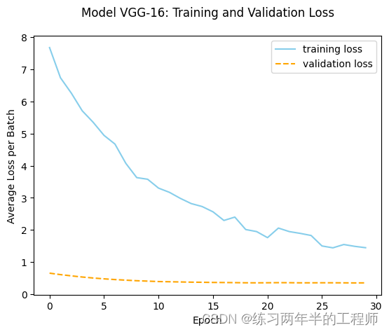
9. 绘画VGG训练和验证损失的曲线图

plt.figure()
vgg_train_loss = history_vgg['train_loss']
vgg_val_loss = history_vgg['val_loss']
vgg_epoch = range(0, len(vgg_train_loss), 1)
plot3, = plt.plot(vgg_epoch, vgg_train_loss, linestyle = "solid", color = "skyblue")
plot4, = plt.plot(vgg_epoch, vgg_val_loss, linestyle = "dashed", color = "orange")
plt.legend([plot3, plot4], ['training loss', 'validation loss'])
plt.xlabel('Epoch')
plt.ylabel('Average Loss per Batch')
plt.title('Model VGG-16: Training and Validation Loss', pad = 20)
plt.savefig('VGG16-Loss-Plot.png')
1
2
3
4
5
6
7
8
9
10
11

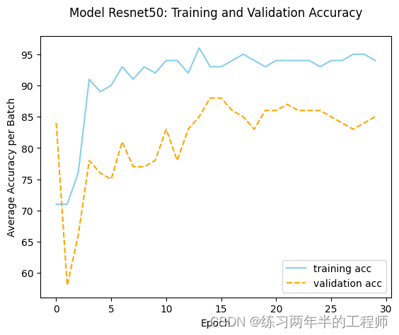
10. 绘画Resnet训练和验证准确率的曲线图

# Training Reseults: Resnet50
plt.figure()
resnet50_train_acc = history_resnet50['train_acc']
resnet50_val_acc = history_resnet50['val_acc']
resnet50_epoch = range(0, len(resnet50_train_acc), 1)
plot5, = plt.plot(resnet50_epoch, resnet50_train_acc, linestyle = "solid", color = "skyblue")
plot6, = plt.plot(resnet50_epoch, resnet50_val_acc, linestyle = "dashed", color = "orange")
plt.legend([plot5, plot6], ['training acc', 'validation acc'])
plt.xlabel('Epoch')
plt.ylabel('Average Accuracy per Batch')
plt.title('Model Resnet50: Training and Validation Accuracy', pad = 20)
plt.savefig('Resnet50-Acc-Plot.png')
1
2
3
4
5
6
7
8
9
10
11
12

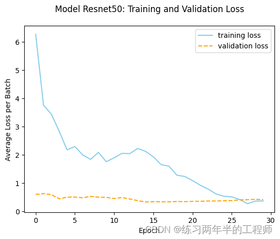
11. 绘画Resnet训练和验证损失的曲线图

plt.figure()
resnet50_train_loss = history_resnet50['train_loss']
resnet50_val_loss = history_resnet50['val_loss']
resnet50_epoch = range(0, len(resnet50_train_loss), 1)
plot7, = plt.plot(resnet50_epoch, resnet50_train_loss, linestyle = "solid", color = "skyblue")
plot8, = plt.plot(resnet50_epoch, resnet50_val_loss, linestyle = "dashed", color = "orange")
plt.legend([plot7, plot8], ['training loss', 'validation loss'])
plt.xlabel('Epoch')
plt.ylabel('Average Loss per Batch')
plt.title('Model Resnet50: Training and Validation Loss', pad = 20)
plt.savefig('Resnet50-Loss-Plot.png')
1
2
3
4
5
6
7
8
9
10
11

12. 绘画验证损失的比较图

plt.figure()
df_valid_loss = pd.DataFrame({'Epoch': range(0, N_EPOCHS, 1),
                       'valid_loss_vgg': history_vgg['val_loss'],
                       'valid_loss_resnet50':history_resnet50['val_loss']
                       })
plota, = plt.plot('Epoch', 'valid_loss_vgg', data=df_valid_loss, linestyle = '--', color = 'skyblue')
plotb, = plt.plot('Epoch', 'valid_loss_resnet50', data=df_valid_loss, color = 'orange')
plt.xlabel('Epoch')
plt.ylabel('Average Validation Loss per Batch')
plt.title('Validation Loss Comparison', pad = 20)
plt.legend([plota, plotb], ['VGG16', 'Resnet50'])
plt.savefig('Result_Comparison.png')
1
2
3
4
5
6
7
8
9
10
11
12

13. 定义并执行预测函数

def predict(mymodel, model_name_pt, loader):

    model = mymodel
    model.load_state_dict(torch.load(model_name_pt))
    model.to(device)
    model.eval()
    y_actual_np = []
    y_pred_np = []
    for idx, data in enumerate(loader):
        test_x, test_label = data[0], data[1]
        test_x = test_x.to(device)
        y_actual_np.extend(test_label.cpu().numpy().tolist())

        with torch.no_grad():
            y_pred_logits = model(test_x)
            pred_labels = np.argmax(y_pred_logits.cpu().numpy(), axis=1)
            print("Predicting ---->", pred_labels)
            y_pred_np.extend(pred_labels.tolist())

    return y_actual_np, y_pred_np

y_actual_vgg, y_predict_vgg = predict(model_vgg, "model_vgg.pt", test_loader)
y_actual_resnet50, y_predict_resnet50 = predict(model_resnet50, "model_resnet50.pt", test_loader)
1
2
3
4
5
6
7
8
9
10
11
12
13
14
15
16
17
18
19
20
21
22
23

14. 计算VGG的准确性和混淆矩阵

# VGG-16 Accuracy
print("=====================================================")
acc_rate_vgg = 100*accuracy_score(y_actual_vgg, y_predict_vgg)
print("The Accuracy rate for the VGG-16 model is: ", acc_rate_vgg)
# Confusion matrix for model-VGG-16
print("The Confusion Matrix for VGG-16 is as below:")
print(confusion_matrix(y_actual_vgg, y_predict_vgg))
1
2
3
4
5
6
7

输出为：

The Accuracy rate for the VGG-16 model is: 88.16666666666667
The Confusion Matrix for VGG-16 is as below:
[[7106 894]
[ 171 829]]

15. 计算Resnet的准确性和混淆矩阵

print("=====================================================")
acc_rate_resnet50 = 100*accuracy_score(y_actual_resnet50, y_predict_resnet50)
print("The Accuracy rate for the Resnet50 model is: ", acc_rate_resnet50)
# Confusion matrix for model Resnet50
print("The Confusion Matrix for Resnet50 is as below:")
print(confusion_matrix(y_actual_resnet50, y_predict_resnet50))
1
2
3
4
5
6

输出为：

The Accuracy rate for the Resnet50 model is: 85.35555555555555
The Confusion Matrix for Resnet50 is as below:
[[6843 1157]
[ 161 839]]