机器学习——决策树与随机森林

机器学习——决策树与随机森林

---

前言

决策树和随机森林都是常见的机器学习算法，用于分类和回归任务，本文将对这两种算法进行介绍。

---

一、决策树

1.1. 原理

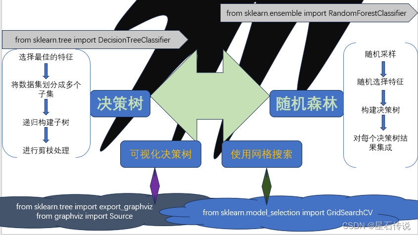
决策树算法是一种基于树结构的分类和回归算法。它通过对数据集进行递归地二分，选择最佳的特征进行划分，直到达到终止条件。
决策树的每个内部节点表示一个特征，根据测试结果进行分类，每个叶子节点表示一个类别或一个回归值。
决策树的构建可以通过以下几个步骤来实现：

1. 特征选择：根据某个评价指标（如信息增益、基尼不纯度等），选择最佳的特征作为当前节点的划分特征。（即哪个特征带来最多的信息变化幅度，就选择哪一个特征来分类）

2. 划分数据集：根据选择的特征，将数据集划分成多个子集，每个子集对应一个分支。对于离散特征，可以根据特征值的不同进行划分；对于连续特征，可以选择一个阈值进行划分。

3. 递归构建子树：对每个子集递归地构建子树，直到所有子集被正确分类或满足终止条件。常见的终止条件有：达到最大深度、样本数量小于阈值、节点中的样本属于同一类别等。

4. 避免过拟合：对决策树进行剪枝处理。剪枝可以分为前剪枝和后剪枝： 前剪枝是在构建树的过程中进行剪枝，通过设定一个阈值，信息熵减小的数量小于这个值则停止创建分支；后剪枝则是在决策树构建完成后，对节点检查其信息熵的增益来判断是否进行剪枝。
   还可以通过控制决策树的最大深度（max_depth）

1.2. 代码实现

import numpy as np
from sklearn.datasets import make_moons
from sklearn.model_selection import train_test_split
from sklearn.tree import DecisionTreeClassifier

#生成数据集
np.random.seed(41)
raw_data = make_moons(n_samples=2000, noise=0.25, random_state=41)
data = raw_data[0]
target = raw_data[1]

# 训练决策树分类模型
x_train, x_test, y_train, y_test = train_test_split(data, target)
classifer = DecisionTreeClassifier()
classifer.fit(x_train, y_train)
#计算测试数据集在决策树模型上的准确率得分
print(classifer.score(x_test, y_test))
0.916


# max_depth 树的最大深度，默认为None
classifer = DecisionTreeClassifier(max_depth=6)
classifer.fit(x_train, y_train)
print(classifer.score(x_test, y_test))
0.934

# min_samples_leaf 叶节点所需的最小样本数,默认为1
classifer = DecisionTreeClassifier(max_depth=6, min_samples_leaf=6)
classifer.fit(x_train, y_train)
print(classifer.score(x_test, y_test))
0.938


# min_impurity_decrease 划分节点时的最小信息增益
def m_score(value):
    model = DecisionTreeClassifier(min_impurity_decrease=value)
    model.fit(x_train, y_train)
    train_score = model.score(x_train, y_train)
    test_score = model.score(x_test, y_test)
    return train_score, test_score
values = np.linspace(0,0.01,50)
score = [m_score(value) for value in values ]
train_s = [s[0] for s in score]
test_s = [s[1] for s in score]
best_index = np.argmax(test_s)
print(test_s[best_index])
print(values[best_index])
plt.plot(train_s,label = "train_s")
plt.plot(test_s,label = "test_s")
plt.legend()
plt.show()
1
2
3
4
5
6
7
8
9
10
11
12
13
14
15
16
17
18
19
20
21
22
23
24
25
26
27
28
29
30
31
32
33
34
35
36
37
38
39
40
41
42
43
44
45
46
47
48
49
50
51

从以上代码中可以看出在不同参数的选择情况下，准确率（分类器预测正确的样本数量与总样本数量的比例）得分是不同的，越接近1表示模型的预测性能越好

1.3. 网格搜索

可以使用网格搜索获得最优的模型参数：

# 使用网格搜索获得最优的模型参数
from sklearn.model_selection import GridSearchCV
classifer = DecisionTreeClassifier()
params = {
    "max_depth": np.arange(1, 10),
    "min_samples_leaf": np.arange(1, 20),
    "min_impurity_decrease": np.linspace(0,0.4,50),
    "criterion" : ("gini","entropy")
}
grid_searchcv = GridSearchCV(classifer, param_grid=params, scoring="accuracy",
                             cv=5)  # scoring指定模型评估指标，例如：'accuracy'表示使用准确率作为评估指标。
grid_searchcv.fit(x_train, y_train)
print(grid_searchcv.best_params_)
print(grid_searchcv.best_score_)
#print(grid_searchcv.cv_results_)
print(grid_searchcv.best_index_)
print(grid_searchcv.best_estimator_)
best_clf = grid_searchcv.best_estimator_
best_clf.fit(x_train,y_train)
print(best_clf.score(x_test,y_test))
#结果：
{'criterion': 'entropy', 'max_depth': 8, 'min_impurity_decrease': 0.0, 'min_samples_leaf': 16}
0.9286666666666668
15215
DecisionTreeClassifier(criterion='entropy', max_depth=8, min_samples_leaf=16)
0.94
1
2
3
4
5
6
7
8
9
10
11
12
13
14
15
16
17
18
19
20
21
22
23
24
25
26
27

1.4. 可视化决策树

得到可视化决策树文件：

df = pd.DataFrame(data = data,columns=["x1","x2"])
from sklearn.tree import export_graphviz
from graphviz import Source
dot_data = export_graphviz(best_clf, out_file=None, feature_names=df.columns)
graph = Source(dot_data)
graph.format = 'png'file
graph.render(filename='file_image', view=True)

1
2
3
4
5
6
7
8

二、随机森林算法

2.1. 原理

随机森林是一种集成学习方法，它通过构建多个决策树来进行分类或回归，
随机森林的基本原理：

1. 随机采样：从原始训练集中随机选择一定数量的样本，作为每个决策树的训练集。

2. 随机特征选择：对于每个决策树的每个节点，从所有特征中随机选择一部分特征进行评估，选择最佳的特征进行划分。

3. 构建决策树：根据随机采样和随机特征选择的方式，构建多个决策树。

4. 预测：对于分类问题，通过投票或取平均值的方式，将每个决策树的预测结果进行集成；对于回归问题，将每个决策树的预测结果取平均值。

随机森林函数中的超参数：

1. n_estimators：它表示随机森林中决策树的个数。

2. min_samples_split：内部节点分裂所需的最小样本数

3. min_samples_leaf：叶节点所需的最小样本数

4. max_features：每个决策树考虑的最大特征数量

5. n_jobs ：表示允许使用处理器的数量

6. criterion ：gini 或者entropy (default = gini)

7. random_state：随机种子

2.2. 代码实现

import numpy as np
import pandas as pd
from sklearn.datasets import make_moons
from sklearn.model_selection import train_test_split
from sklearn.ensemble import RandomForestClassifier
#训练随机森林分类模型
np.random.seed(42)
raw_data = make_moons(n_samples= 2000,noise= 0.25,random_state=42)
data,target = raw_data[0],raw_data[1]

x_train, x_test, y_train, y_test = train_test_split(data, target,random_state=42)
classfier = RandomForestClassifier(random_state= 42)
classfier.fit(x_train,y_train)
score = classfier.score(x_test,y_test)
print(score)
0.93




#网格搜索获取最优参数
from sklearn.model_selection import GridSearchCV
param_grids = {
    "criterion": ["gini","entropy"],
    "max_depth":np.arange(1,10),
    "min_samples_leaf":np.arange(1,10),
    "max_features": np.arange(1,3)
}
grid_search = GridSearchCV(RandomForestClassifier(),param_grid=param_grids,n_jobs= 1,scoring="accuracy",cv=5)
grid_search.fit(x_train,y_train)
print(grid_search.best_params_)  #最优的参数
print(grid_search.best_score_)	#最好的得分
best_clf = grid_search.best_estimator_   #最优的模型
print(best_clf)
best_clf.fit(x_train,y_train)
print(best_clf.score(x_test,y_test))  #查看测试集在最优模型上的得分
#结果：
{'criterion': 'entropy', 'max_depth': 9, 'max_features': 1, 'min_samples_leaf': 7}
0.9506666666666665
RandomForestClassifier(criterion='entropy', max_depth=9, max_features=1,
                       min_samples_leaf=7)
0.932

1
2
3
4
5
6
7
8
9
10
11
12
13
14
15
16
17
18
19
20
21
22
23
24
25
26
27
28
29
30
31
32
33
34
35
36
37
38
39
40
41
42
43

三、补充（过拟合与欠拟合）

过拟合指的是模型在训练集上表现得很好，但在测试集或新数据上表现不佳的情况。
过拟合通常发生在模型过于复杂或训练数据过少的情况下

欠拟合指的是模型无法很好地拟合训练集，导致在训练集和测试集上的误差都很高。
欠拟合通常发生在模型过于简单或训练数据过于复杂的情况下

---

总结

总之，决策树和随机森林都是基于树结构的机器学习算法，具有可解释性和特征选择的能力。随机森林是多个决策树的集成模型，引入了随机性并通过投票或平均来得出最终预测结果，可以有效降低噪声干扰，提高模型的准确性与稳定性，但是增加了计算量。

锦帽貂裘，千骑卷平冈

–2023-9-1 筑基篇