迁移学习（COAL）《Generalized Domain Adaptation with Covariate and Label Shift CO-ALignment》

论文信息

论文标题：Generalized Domain Adaptation with Covariate and Label Shift CO-ALignment
论文作者：Shuhan Tan, Xingchao Peng, Kate Saenko
论文来源：ICLR 2020
论文地址：download 
论文代码：download
视屏讲解：click

1 摘要

　　提出问题：标签偏移；

　　解决方法：

　　　　原型分类器模拟类特征分布，并使用 Minimax Entropy 实现条件特征对齐；

　　　　使用高置信度目标样本伪标签实现标签分布修正；

2 介绍

2.1 当前工作

　　假设条件标签分布不变 p(y∣x)=q(y∣x)" role="presentation">p(y∣x)=q(y∣x)$p(y\mid x)=q(y\mid x)$，只有特征偏移 p(x)≠q(x)" role="presentation">p(x)≠q(x)$p(x)\ne q(x)$，忽略标签偏移 p(y)≠q(y)" role="presentation">p(y)≠q(y)$p(y)\ne q(y)$。

　　假设不成立的原因：

• • 场景不同，标签跨域转移 p(y)≠q(y)" role="presentation">p(y)≠q(y)$p(y)\ne q(y)$ 很常见；
  • 如果存在标签偏移，则当前的 UDA 工作性能显著下降；
  • 一个合适的 UDA 方法应该能同时处理协变量偏移和标签偏移；

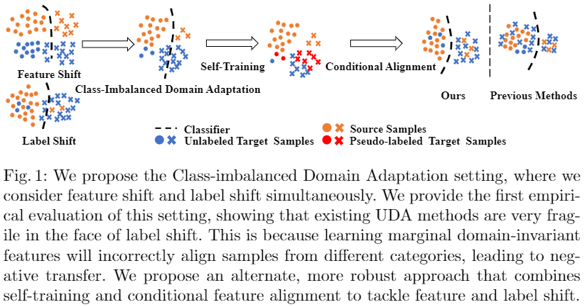
2.2 本文工作

　　本文提出类不平衡域适应 (CDA)，需要同时处理 条件特征转移 和 标签转移。

　　具体来说，除了协变量偏移假设 p(x)≠q(x)" role="presentation">p(x)≠q(x)$p(x)\ne q(x)$, p(y∣x)=q(y∣x)" role="presentation">p(y∣x)=q(y∣x)$p(y\mid x)=q(y\mid x)$，进一步假设 p(x∣y)≠q(x∣y)" role="presentation">p(x∣y)≠q(x∣y)$p(x\mid y)\ne q(x\mid y)$ 和 p(y)≠q(y)" role="presentation">p(y)≠q(y)$p(y)\ne q(y)$。

　　CDA 的主要挑战：

• • 标签偏移阻碍了主流领域自适应方法的有效性，这些方法只能边缘对齐特征分布；
  • 在存在标签偏移的情况下，对齐条件特征分布 p(x∣y)" role="presentation">p(x∣y)$p(x\mid y)$, q(x∣y)" role="presentation">q(x∣y)$q(x\mid y)$ 很困难；
  • 当一个或两个域中的数据在不同类别中分布不均时，很难训练无偏分类器；

　　CDA 概述：

　　

3 问题定义

　　In Class-imbalanced Domain Adaptation, we are given a source domain  DS={(xis,yis)i=1Ns}" role="presentation">DS={(xsi,ysi)Nsi=1}${\mathcal{D}}_{\mathcal{S}}=\left\{{(x_i^s,y_i^s)}_{i=1}^{N_s}\right\}$  with  Ns" role="presentation">Ns$N_s$  labeled examples, and a target domain  DT={(xit)i=1Nt}" role="presentation">DT={(xti)Nti=1}${\mathcal{D}}_{\mathcal{T}}=\left\{{\left(x_i^t\right)}_{i=1}^{N_t}\right\}$  with  Nt" role="presentation">Nt$N_t$  unlabeled examples. We assume that  p(y∣x)=q(y∣x)" role="presentation">p(y∣x)=q(y∣x)$p(y\mid x)=q(y\mid x)$  but  p(x∣y)≠q(x∣y)" role="presentation">p(x∣y)≠q(x∣y)$p(x\mid y)\ne q(x\mid y)$, p(x)≠q(x)" role="presentation">p(x)≠q(x)$p(x)\ne q(x)$ , and  p(y)≠q(y)" role="presentation">p(y)≠q(y)$p(y)\ne q(y)$ . We aim to construct an end-to-end deep neural network which is able to transfer the knowledge learned from  DS" role="presentation">DS${\mathcal{D}}_{\mathcal{S}}$  to  DT" role="presentation">DT${\mathcal{D}}_{\mathcal{T}}$ , and train a classifier  y=θ(x)" role="presentation">y=θ(x)$y=\theta (x)$  which can minimize task risk in target domain  ϵT(θ)=Pr(x,y)∼q⁡[θ(x)≠y]" role="presentation">ϵT(θ)=Pr(x,y)∼q[θ(x)≠y]${ϵ}_T(\theta )={\mathrm{Pr}}_{(x,y)\sim q}[\theta (x)\ne y]$. 

4 方法

4.1 整体框架

　　

4.2 用于特征转移的基于原型的条件对齐

　　目的：对齐 p(x∣y)" role="presentation">p(x∣y)$p(x\mid y)$ 和 q(x∣y)" role="presentation">q(x∣y)$q(x\mid y)$

　　步骤：首先使用原型分类器（基于相似度）估计 p(x∣y)" role="presentation">p(x∣y)$p(x\mid y)$ ，然后使用一种 minimax entropy" role="presentation">minimax entropy$\text{minimax entropy}$ 算法将其和 q(x∣y)" role="presentation">q(x∣y)$q(x\mid y)$ 对齐；

4.2.1 原型分类器

　　原因：基于原型的分类器在少样本学习设置中表现良好，因为在标签偏移的假设下中，某些类别的设置频率可能较低；

python

# 深层原型分类器
class Predictor_deep_latent(nn.Module):
    def __init__(self, in_dim = 1208, num_class = 2, temp = 0.05):
        super(Predictor_deep_latent, self).__init__()
        self.in_dim = in_dim
        self.hid_dim = 512
        self.num_class = num_class
        self.temp = temp  #0.05

        self.fc1 = nn.Linear(self.in_dim, self.hid_dim)
        self.fc2 = nn.Linear(self.hid_dim, num_class, bias=False)

    def forward(self, x, reverse=False, eta=0.1):
        x = self.fc1(x)
        if reverse:
            x = GradReverse.apply(x, eta)
        feat = F.normalize(x)
        logit = self.fc2(feat) / self.temp
        return feat, logit

　　源域上的样本使用交叉熵做监督训练：

　　　　LSC=E(x,y)∈DSLce(h(x),y)(1)" role="presentation">LSC=E(x,y)∈DSLce(h(x),y)(1)${\mathcal{L}}_{SC}={\mathbb{E}}_{(x,y)\in {\mathcal{D}}_S}{\mathcal{L}}_{ce}(h(x),y)(1)$

　　样本 x" role="presentation">x$x$ 被分类为 i" role="presentation">i$i$ 类的置信度越高，x" role="presentation">x$x$ 的嵌入越接近 wi" role="presentation">wi$w_i$。因此，在优化上式时，通过将每个样本 x" role="presentation">x$x$ 的嵌入更接近其在 W" role="presentation">W$W$ 中的相应权重向量来减少类内变化。所以，可以将 wi" role="presentation">wi$w_i$ 视为 p" role="presentation">p$p$ 的代表性数据点（原型） p(x∣y=i)" role="presentation">p(x∣y=i)$p(x\mid y=i)$ 。

4.2.2 通过 Minimax Entropy 实现条件对齐

　　目标域缺少数据标签，所以使用 Eq.1" role="presentation">Eq.1$\text{Eq.1}$ 获得类原型是不可行的；

　　解决办法：

• • 将每个源原型移动到更接近其附近的目标样本；
  • 围绕这个移动的原型聚类目标样本；

　　因此，提出 熵极小极大 实现上述两个目标。

　　具体来说，对于输入网络的每个样本 xt∈DT" role="presentation">xt∈DT$x^t\in {\mathcal{D}}_{\mathcal{T}}$，可以通过下式计算分类器输出的平均熵

　　　　LH=Ex∈DTH(x)=−Ex∈DT∑i=1chi(x)log⁡hi(x)(2)" role="presentation">LH=Ex∈DTH(x)=−Ex∈DT∑ci=1hi(x)loghi(x)(2)${\mathcal{L}}_H={\mathbb{E}}_{x\in {\mathcal{D}}_{\mathcal{T}}}H(x)=-{\mathbb{E}}_{x\in {\mathcal{D}}_{\mathcal{T}}}\sum _{i=1}^c{h}_i(x)\log h_i(x)(2)$

　　通过在对抗过程中对齐源原型和目标原型来实现条件特征分布对齐：

• • 训练 C" role="presentation">C$C$ 以最大化 LH" role="presentation">LH${\mathcal{L}}_H$ ，旨在将原型从源样本移动到邻近的目标样本；
  • 训练 F" role="presentation">F$F$ 来最小化 LH" role="presentation">LH${\mathcal{L}}_H$，目的是使目标样本的嵌入更接近它们附近的原型；

4.3 标签转移的类平衡自训练

　　由于源标签分布 p(y)" role="presentation">p(y)$p(y)$ 与目标标签分布 q(y)" role="presentation">q(y)$q(y)$ 不同，因此不能保证在 DS" role="presentation">DS${\mathcal{D}}_{\mathcal{S}}$ 上具有低风险的分类器 C" role="presentation">C$C$ 在 DT" role="presentation">DT${\mathcal{D}}_{\mathcal{T}}$ 上具有低错误。 直观地说，如果分类器是用不平衡的源数据训练的，决策边界将由训练数据中最频繁的类别主导，导致分类器偏向源标签分布。 当分类器应用于具有不同标签分布的目标域时，其准确性会降低，因为它高度偏向源域。

　　为解决这个问题，本文使用[19]中的方法进行自我训练来估计目标标签分布并细化决策边界。自训练为了细化决策边界，本文建议通过自训练来估计目标标签分布。 我们根据分类器 C" role="presentation">C$C$ 的输出将伪标签 y" role="presentation">y$y$ 分配给所有目标样本。由于还对齐条件特征分布 p(x∣y" role="presentation">p(x∣y$p(x\mid y$ 和 q(x∣y)" role="presentation">q(x∣y)$q(x\mid y)$，假设分布高置信度伪标签 q(y)" role="presentation">q(y)$q(y)$ 可以用作目标域的真实标签分布 q(y)" role="presentation">q(y)$q(y)$ 的近似值。 在近似的目标标签分布下用这些伪标记的目标样本训练 C" role="presentation">C$C$，能够减少标签偏移的负面影响。

　　为了获得高置信度的伪标签，对于每个类别，本文选择属于该类别的具有最高置信度分数的目标样本的前 k" role="presentation">k$k$。利用 h(x)" role="presentation">h(x)$h(x)$ 中的最高概率作为分类器对样本 x" role="presentation">x$x$ 的置信度。 具体来说，对于每个伪标记样本 (x,y)" role="presentation">(x,y)$(x,y)$，如果 h(x)" role="presentation">h(x)$h(x)$ 位于具有相同伪标签的所有目标样本的前 k" role="presentation">k$k$ 中，将其选择掩码设置为 m=1" role="presentation">m=1$m=1$，否则 m=0" role="presentation">m=0$m=0$。将伪标记目标集表示为 D^T={(xit,y^it,mi)i=1Nt}" role="presentation">D^T={(xti,y^ti,mi)Nti=1}${\hat{\mathcal{D}}}_T=\left\{{(x_i^t,{\hat{y}}_i^t,m_i)}_{i=1}^{N_t}\right\}$，利用来自 D^T" role="presentation">D^T${\hat{\mathcal{D}}}_T$ 的输入和伪标签来训练分类器 C" role="presentation">C$C$，旨在细化决策 与目标标签分布的边界。 分类的总损失函数为：

　　　　LST=LSC+E(x,y^,m)∈D^TLce(h(x),y^)⋅m" role="presentation">LST=LSC+E(x,y^,m)∈D^TLce(h(x),y^)⋅m${\mathcal{L}}_{ST}={\mathcal{L}}_{SC}+{\mathbb{E}}_{(x,\hat{y},m)\in {\hat{\mathcal{D}}}_T}{\mathcal{L}}_{ce}(h(x),\hat{y})\cdot m$

　　通常，用 k0=5" role="presentation">k0=5$k_0=5$ 初始化 k" role="presentation">k$k$，并设置 kstep =5" role="presentation">kstep =5$k_{\text{step }}=5$，kmax=30" role="presentation">kmax=30$k_{max}=30$。

　　Note：本文还对源域数据使用了平衡采样的方法，使得分类器不会偏向于某一类。

4.4 训练目标

　　总体目标：

　　　　C^=arg⁡minCLST−αLHF^=arg⁡minFLST+αLH" role="presentation">C^=argminCLST−αLHF^=argminFLST+αLH$\begin{array}{l}\hat{C}=\underset{C}{\arg min}{\mathcal{L}}_{ST}-\alpha {\mathcal{L}}_H\\ \hat{F}=\underset{F}{\arg min}{\mathcal{L}}_{ST}+\alpha {\mathcal{L}}_H\end{array}$

5 总结

　　略

• 论文信息
• 1 摘要
• 2 介绍
•     2.1 当前工作
•     2.2 本文工作
• 3 问题定义
• 4 方法
•     4.1 整体框架
•     4.2 用于特征转移的基于原型的条件对齐
•         4.2.1 原型分类器
•         4.2.2 通过 Minimax Entropy 实现条件对齐
•     4.3 标签转移的类平衡自训练
•     4.4 训练目标
• 5 总结

__EOF__