【Python自然语言处理】文本向量化处理用户对不同类型服装评论问题（超详细 附源码）

需要源码和数据集请点赞关注收藏后评论区留言私信~~~

下面以文本向量化为目标，举例说明基于不同模型的实现过程，使用的数据集的主题是用户对不同类型的女性服装的评论，总共有23485条记录 实现步骤如下

一、导入库文件

首先导入需要的库文件，本实例设计词频-逆文档模型，N元模型以及词袋模型，并利用混淆矩阵直观描述各模型的预测能力 代码如下

import gensim
import nltk
from sklearn.model_selection import train_test_split
from sklearn import linear_model
from sklearn.neighbors import KNeighborsClassifier
from sklearn import linear_model
from nltk.corpus import stopwords
from sklearn.feature_extraction.text import CountVectorizer, TfidfVectorizer
from sklearn.metrics import accuracy_score, confusion_matrix
import matplotlib.pyplot as plt
from gensim.models import Word2Vec
import logging
from smart_open import smart_open
import pandas as pd
import numpy as np
from numpy import random

二、数据清洗 

读入评论数据，删除空值，以空格符为基准对用户评论进行统计，针对数据的评论列进行分类统计，只分析用户关注度高且排名前五的用户评论，得到分类统计的图形比较结果如下

 

 三、配置混淆矩阵

定义混淆矩阵以及参数设置并设定图形输出的主要特征 代码如下

def confusion_matrix_definition(cm, title='混淆矩阵', cmap=plt.cm.Purples,ax=ax):
    plt.imshow(cm, interpolation='nearest', vmin = -1, vmax = 1, cmap=cmap, origin ='lower')
    plt.title(title,fontweight ="bold")
    plt.colorbar(plt.imshow(cm, interpolation='nearest', cmap=cmap, origin ='lower'))
    length = np.arange(len(categories))
    plt.xticks(length, categories, rotation=45)
    plt.yticks(length, categories)
    plt.rcParams['font.sans-serif']=['Microsoft YaHei']
    plt.rcParams['font.size']=14
    plt.rcParams['axes.unicode_minus'] = False
    plt.ylabel('真实值')
    plt.xlabel('预测值')
    #plt.tight_layout()
    plt.show()

四、预测结果

评估预测结果，通过正则化混淆矩阵方式显示预测值和期望值之间的关系，以客户评论数据为预测对象，选取排名前五的女性服饰类型，调用评估预测函数得到评估结果，并且剔除长度不符合要求的数据

五、结果展示

词袋模型结果

 

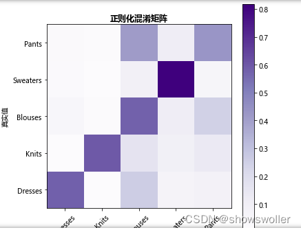
 由上图可知，对角线上的值表示正确分类的结果，颜色越深数字越大，分类结果越正确，非对角线上的值表示模型错误分类结果，颜色越深数值越大，被错误分类的概率越大，可见模型对Sweaters类型的预测分类结果准确性最高，其他略低。 

N元模型结果 

N元模型的混淆矩阵评估结果如下图，分类最为准确的依然是Sweaters，其次是Blouses，而其他三种类型的预估结果比较接近，整个模型的准确性比词袋模型高，可以达到差不多0.7

词频-逆文档频率模型 

词频-逆文档模型评估结果如下 预测精度的顺序基本没有改变

六、总结 

从上面的实例中可以看出，分别使用三种文本向量评估模型，Sweaters的分类结果相对准确，Blouses准确性次之，而其他三种准确性相差不大，模型整体准确率而言，从高到低的顺序依次为N元模型，词袋模型以及词频-逆文档模型，因此针对不同的文本信息处理，不同的模型可能在评价结果的准确性排序上存在一定差异，准确性精度也可能有所区别

七、代码

 
 
 
 
#导入各类库
import gensim
import nltk
from sklearn.model_selection import train_test_split
from sklearn import linear_model
from sklearn.neighbors import KNeighborsClassifier
from sklearn import linear_model
from nltk.corpus import stopwords
from sklearn.feature_extraction.text import CountVectorizer, TfidfVectorizer
from sklearn.metrics import accuracy_score, confusion_matrix
import matplotlib.pyplot as plt
from gensim.models import Word2Vec
import logging
from smart_open import smart_open
import pandas as pd
import numpy as np
from numpy import random
 
 
get_ipython().run_line_magic('matplotlib', 'inline')
 
 
# 统计数据特征
# 
# 
 
# In[2]:
 
 
#读入数据
df = pd.read_csv('data/Reviews.csv')
df = df.dropna()
df['review'].apply(lambda y: len(y.split(' '))).sum()
 
 
# In[3]:
 
 
#分类
#categories = ['Intimates' , 'Dresses', 'Pants', 'Blouses', 'Knits', 'Lounge', 'Jackets', 'Outwear','Skirts', 'Swim', 'Sleep','Fine gauge','Trend','Jeans','Blouses','Casual bottoms','Chemises','Layering','Legwear','Shorts']
 
categories = ['Dresses', 'Knits', 'Blouses', 'Sweaters', 'Pants']
 
 
df=df.groupby('category').filter(lambda x : len(x)>1000)
#df=df.groupby(["category"]).get_group("Dresses", "Knits")
 
#df=df[df['category'].value_counts()<1000]
 
 
ax =df.category.value_counts().head(5).plot(kind="bar",figsize=(30,12),fontsize=35)
ax.set_xlabel("服装类型",fontsize=35,fontfamily='Microsoft YaHei')
ax.set_ylabel("频率统计",fontsize=35,fontfamily='Microsoft YaHei')
#df=df['category'].value_counts(ascending=False).loc[lambda x : x>1000]
print(df)
 
 
# In[4]:
 
 
#df
 
 
# In[5]:
 
 
def plot(indx):
    inx = df[df.index == indx][['review', 'category']].values[0]
    if len(inx) > 5:
        print(inx[0])
        print('Type:', inx[1])
 
 
# In[6]:
 
 
train_data, test_data = train_test_split(df, test_size=0.2, random_state=32)
 
 
# In[7]:
 
 
len(test_data)
 
 
# In[8]:
 
 
plt.figure(figsize=(30, 10))
test_data.category.value_counts().head(5).plot(kind="bar", figsize=(30,12),fontsize=35)
 
print(test_data)
print(test_data['review'])
 
 
# ## Model evaluation approach
# We will use confusion matrices to evaluate all classifiers
 
# In[9]:
 
 
def confusion_matrix_definition(cm, title='混淆矩阵', cmap=plt.cm.Purples,ax=ax):
    plt.imshow(cm, interpolation='nearest', vmin = -1, vmax = 1, cmap=cmap, origin ='lower')
    plt.title(title,fontweight ="bold")
    plt.colorbar(plt.imshow(cm, interpolation='nearest', cmap=cmap, origin ='lower'))
    length = np.arange(len(categories))
    plt.xticks(length, categories, rotation=45)
    plt.yticks(length, categories)
    plt.rcParams['font.sans-serif']=['Microsoft YaHei']
    plt.rcParams['font.size']=14
    plt.rcParams['axes.unicode_minus'] = False
    plt.ylabel('真实值')
    plt.xlabel('预测值')
    #plt.tight_layout()
    plt.show()
 
 
 
 
# In[10]:
 
 
def predict_appraise(predict, mark, title="混淆矩阵"):
    print('准确率： %s' % accuracy_score(mark, predict))
    cm = confusion_matrix(mark, predict)
    
    N = len(cm[0])
    for i in range(N // 2):
        for j in range(i, N - i - 1):
            temp = cm[i][j]
            cm[i][j] = cm[N - 1 - j][i]
            cm[N - 1 - j][i] = cm[N - 1 - i][N - 1 - j]
            cm[N - 1 - i][N - 1 - j] = cm[j][N - 1 - i]
            cm[j][N - 1 - i] = temp
 
    print('混淆矩阵：\n %s' % cm)
    print('(行=期望值, 列=预测值)')
    
    for i in range(N // 2):
        for j in range(i, N - i - 1):
            temp = cm[i][j]
            cm[i][j] = cm[N - 1 - j][i]
            cm[N - 1 - j][i] = cm[N - 1 - i][N - 1 - j]
            cm[N - 1 - i][N - 1 - j] = cm[j][N - 1 - i]
            cm[j][N - 1 - i] = temp
    
    
    cmn = cm.astype('float') / cm.sum(axis=1)[:, np.newaxis]
    fig, ax = plt.subplots(figsize=(6, 6))
    confusion_matrix_definition(cmn, "正则化混淆矩阵")
 
 
# In[11]:
 
 
def predict(vectorizer, classifier, data):
    vt = vectorizer.transform(data['review'])
    forecast = classifier.predict(vt)
    mark = data['category']
    predict_appraise(forecast, mark)
 
 
# ### Bag of words
 
# In[12]:
 
 
def tokenization(text):
    list = []
    for k in nltk.sent_tokenize(text):
        for j in nltk.word_tokenize(k):
            if len(j) < 5:
                continue
            list.append(j.lower())
    return list
 
 
# In[13]:
 
 
get_ipython().run_cell_magic('time', '', '#文本特征向量化\nbow  = CountVectorizer(\n    analyzer="word",  encoding=\'utf-8\',tokenizer=nltk.word_tokenize,\n    preprocessor=None, decode_error=\'strict\', strip_accents=None,stop_words=\'english\', max_features=4200) \ntrain_data_features = bow.fit_transform(train_data[\'review\'])\n#print(bow.get_feature_names())\n')
 
 
# In[14]:
 
 
get_ipython().run_cell_magic('time', '', "\nreg = linear_model.LogisticRegression(n_jobs=1, C=1e7)\nreg = reg.fit(train_data_features, train_data['category'])\n")
 
 
# In[15]:
 
 
bow.get_feature_names()[80:90]
 
 
# In[16]:
 
 
get_ipython().run_cell_magic('time', '', '\npredict(bow, reg, test_data)\n')
 
 
# In[17]:
 
 
def words_impact_evaluate(vectorizer, genre_index=0, num_words=10):
    features = vectorizer.get_feature_names()
    max_coef = sorted(enumerate(reg.coef_[genre_index]), key=lambda x:x[1], reverse=True)
    return [features[x[0]] for x in max_coef[:num_words]]    
 
 
# In[18]:
 
 
# words for the fantasy genre
id = 1
print(categories[id])
words_impact_evaluate(bow,id)
 
 
# In[19]:
 
 
train_data_features[0]
 
 
# ### Character N-grams
 
# In[1]:
 
 
get_ipython().run_cell_magic('time', '', 'n_gram= CountVectorizer(\n    analyzer="char",\n    ngram_range=([3,6]),\n    tokenizer=None,    \n    preprocessor=None,                               \n    max_features=4200) \n\nreg = linear_model.LogisticRegression(n_jobs=1, C=1e6)\n\ntrain_data_features = n_gram.fit_transform(train_data[\'review\'])\n\nreg = reg.fit(train_data_features, train_data[\'category\'])\n')
 
 
# In[2]:
 
 
n_gram.get_feature_names()[70:90]
 
 
# In[3]:
 
 
predict(n_gram, reg, test_data)
 
 
# ### TF-IDF
# 
# 
 
# In[4]:
 
 
get_ipython().run_cell_magic('time', '', "tf_idf = TfidfVectorizer(\n    min_df=2, tokenizer=nltk.word_tokenize,\n    preprocessor=None, stop_words='english')\ntrain_data_features = tf_idf.fit_transform(train_data['review'])\n\nreg = linear_model.LogisticRegression(n_jobs=1, C=1e6)\nreg = reg.fit(train_data_features, train_data['category'])\n")
 
 
# In[5]:
 
 
tf_idf.get_feature_names()[1000:1010]
 
 
# In[6]:
 
 
predict(tf_idf, reg, test_data)
 
 
# In[ ]:
 
 
words_impact_evaluate(tf_idf, 1)
 

 创作不易 觉得有帮助请点赞关注收藏~~~