-
Jitter
1、Jitter定义
定义1(SONET规范):抖动可以定义为数字信号在重要时点上偏离理想时间位置的短期变化。
2、Total Jitter表征方式

2.1、周期抖动(Period Jitter),与理想时钟无关,不累积
Period jitter is defined as the maximum deviation of any clock period from its mean clock period(替代ideal clock period).
测量项目P1、P2和P3表明的周期性抖动用来测量波形中每个时钟周期的时间。这是可以执行的最简单、最直接的测量。通过调节示波器,并对无穷大余辉设置显示结果,可以显示略长于一个完整时钟周期的周期,进而可以估计峰到峰值。如果示波器在第一个边沿上触发(中间电平触发),可以在第二个边沿上查看周期性抖动,如下图所示。

测量实时波形中每个时钟和数据的周期的宽度。这是最早最直接的一种测量抖动的方式。这一指标说明了时钟信号每个周期的变化。
2.1.1、Long term period jitter(K-Cycle jitter or K-Period Jitter),测量Crystal常用
测量由参考点滞后相当数量K个Cycle(一般K去稍大的值,如500~1000)后时钟的抖动值。该抖动参数也是时钟稳定性的一个重要指标。
Period Jitter也就是K=1的Long term period jitter。

2.1.2、测试25MHz Crystal long term period jitter
Step1:如下图连接被测设备(示波器探头电容尽量小),量测的点是crystal 的XI pin,探棒的接地点离测试点越近越好。接地线也尽可能的短,保证接地效果要好。且点在测点上的探棒要固定,防止接触不良造成jitter值不稳定。

Step2:设定positive edge trigger和DC coupling, autoset使整个clock波形在屏幕中间。并调整position 为50%和trigger点约为整个振幅的一半。
Step3:设定delay time to 10us(相当于K=250,如果10us不是被测时钟周期的的整数倍N,则选择10us附近的值; 如11.0592MHz的时钟,选择10.037 us(相当于K=111))
Step4:将水平(200ps)和垂直(10mv)的scale都调制最小。点击[Display] → [Display Persistence] → [Infinite Persistence],打开累积功能。就会观察到下图clock Jitter的抖动
Step5:点击MeasureàWaveform Histogram。水平方向的宽度能完全覆盖jitter抖动的范围即可。但垂直方向的高度越扁越好(推荐2mv)。
Step6:点击[Measurement Setup] → [Histog] → [PK-PK / Std Dev / Hits in Box] → [Statistics] → [off] → [setup] → [Histogram]。选择Hits(≥10khits)/Std Dev/Pk-Pk三个参数来量测jitter

2.2、相邻周期抖动(Cycle-Cycle Jitter),与理想时钟无关,不累积,属于short-term jitter
测量任意两个相邻时钟或数据的周期宽度的变动有多大,通过对周期抖动应用一阶差分运算,可以得到周期间抖动。这个指标在分析锁相环性质的时候具有明显的意义。

2.3、时间间隔误差(Time Interval Error,TIE),与理想时钟有关,且累积
测量时钟或数据的每个活动边沿与其理想位置有多大偏差,它使用参考时钟或时钟恢复提供理想的边沿。TIE在通信系统中特别重要,因为它说明了周期抖动在各个时期的累计效应。
某以太网产品datasheet中的TIE Jitter指标如下:

25KHz to 25MHz:指的是示波器测试TIE Jitter时,打开TIE Bandpass Filter,选择25KHz to 25MHz。
Broadband:指的是示波器测试TIE Jitter时,关闭TIE Bandpass Filter。
2.4、三者关系

备注:上面的图片关于Period Jitter是错误的,显示的是单纯的Period,而不是Period Jitter。


例:某1MHz时钟(1000ns),测得的周期分别为990、990、990、990、1010、1010、1010、1010…
Period
990
990
990
990
1010
1010
1010
1010
1010
1010
1010
1010
990
Period Jitter -10 -10 -10 -10 10 10 10 10 10 10 10 10 -10 Cycle-Cycle Jitter
NA
0
0
0
20
0
0
0
0
0
0
0
-20
TIE Jitter
-10
-20
-30
-40
-30
-20
-10
0
10
20
30
40
30
3、Jitter来源
 ,数值直接相加即可
其中,
DCD是Duty-Cycle Distortion;
DDJ也有称作Pattern-Dependent Jitter,或ISI。
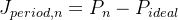
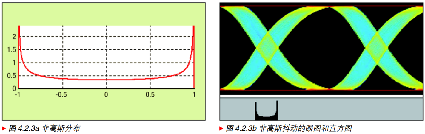
确定性抖动是非高斯分布的,且有界(Bounded)的。

3.1、随机性抖动(Random Jitter):高斯分布

3.2、周期性抖动(Periodic Jitter):正弦函数概率密度,不同于Period Jitter
3.3、数据相关抖动(DDJ):多个独立分布(至少两个)

图中PDF是与随机抖动卷积之后的结果,原本应该是两条竖线。
3.4、占空比相关抖动(DCD):两个独立分布

图中PDF是与随机抖动卷积之后的结果,原本应该是两条竖线。
4、Peak to Peak和Std Dev(RMS)
4.1、Standard deviation is same as RMS(Root Mmean Square),Why?


当平均值
 时,两者相等,而对于随机抖动而言,平均值可以认为等于0。
4.2、Peak-Peak和RMS Random Jitter之间的关系
两者换算的前提是Random Jitter满足高斯分布,另外必须在换算之前框定Probability of Error(如bit error,BER)。

其中,DTD是信号的数据变换密度,对于数据data而言,DTD定义为边沿变化与比特数之间的比率(如sgmii的DTD=0.5,625MHz,1.25G 比特数据);对于时钟clock而言,DTD=1。由上面的公式可以得到波峰因数N。

其中,N是波峰因数(crest factor)。
例如,IEEE 802.3规定1000Base-X BER(Probability of Error)为
1 0 − 12 5、Phase Noise
5.1、jitter和phase noise的关系
- 数字电路:jitter较多
- 模拟电路:phase noise较多
5.2、Phase Noise to Jitter的转化
- function Jitter = Pn2Jitter(f, Lf, fc)
- %
- % Summary: Jitter (RMS) calculation from phase noise vs. frequency data.
- %
- % Calculates RMS jitter by integrating phase noise power data.
- % Phase noise data can be derived from graphical information or an
- % actual measurement data file.
- %
- % Usage:
- % Jitter = Pn2Jitter(f, Lf, fc)
- % Inputs:
- % f: Frequency vector (phase noise break points), in Hz, row or column.
- % Lf: Phase noise vector, in dBc/Hz, same dimensions, size(), as f.
- % fc: Carrier frequency, in Hz, a scalar.
- % Output:
- % Jitter: RMS jitter, in seconds.
- %
- % Examples:
- % [1] >> f = [10^0 10^1 10^3 10^4 10^6]; Lf = [-39 -73 -122 -131 -149];
- % >> Jitter = Pn2Jitter(f, Lf, 70e6)
- % Jitter = 2.3320e-011
- % Comparing fordahl application note AN-02-3{*} and jittertime.com{+}
- % calculations at fc = 70MHz
- % Pn2Jitter.m: 23.320ps
- % AN-02-3 (graphical method): 21.135ps
- % AN-02-3 (numerical method): 24.11ps
- % Aeroflex PN9000 computation: 24.56ps
- % JitterTime.com calculation: 23.32ps
- %
- % {*} fordahl Application Note AN-02-3:
- % "Phase noise to Jitter conversion"
- % http://fordahl.com/images/phasenoise.pdf
- % As of 11 May 2007 it also appears here:
- % http://www.metatech.com.hk/appnote/fordahl/pdf/e_AN-02-3.pdf
- % http://www.metatech.com.tw/doc/appnote-fordahl/e-AN-02-3.pdf
- %
- % {+} JitterTime Consulting LLC web calculator
- % http://www.jittertime.com/resources/pncalc.shtml
- % As of 5 May 2008
- %
- % [2] >> f = [10^2 10^3 10^4 10^5 10^6 10^7 4.6*10^9];
- % >> Lf = [-82 -80 -77 -112 -134 -146 -146 ]; format long
- % >> Jitter = Pn2Jitter(f, Lf, 2.25e9)
- % Jitter = 1.566598599875678e-012
- % Comparing ADI application note{$} calculations at fc = 2.25GHz
- % Pn2Jitter.m: 1.56659859987568ps
- % MT-008: 1.57ps
- % Raltron {&}: 1.56659857673259ps
- % JitterTime: 1.529ps--excluding the (4.6GHz, -146) data point,
- % as 1GHz is the maximum allowed
- % {$} Analog Devices, Inc. (ADI) application note MT-008:
- % "Converting Oscillator Phase Noise to Time Jitter"
- % http://www.analog.com/en/content/0,2886,760%255F%255F91502,00.html
- % {&} Raltron web RMS Phase Jitter calculator:
- % "Convert SSB phase noise to jitter"
- % http://www.raltron.com/cust/tools/osc.asp
- % Note: Raltron is restricted to f(min) = 10Hz;
- % therefore it cannot be used in this example [1].
- %
- % [3] >> f = [10^2 10^3 10^4 200*10^6]; Lf = [-125 -150 -174 -174];
- % >> Jitter = Pn2Jitter(f, Lf, 100e6)
- % Jitter = 6.4346e-014
- % Comparing ADI application note{$} calculations at fc = 100MHz
- % Pn2Jitter.m: 0.064346ps
- % MT-008: 0.064ps
- % JitterTime: 0.065ps
- %
- % Note:
- % f and Lf must be the same length, lest you get an error and this
- % Improbable Result: Jitter = 42 + 42i.
- %
- % (A spreadsheet, noise.xls, is available from Wenzel Associates, Inc. at
- % http://www.wenzel.com, "Allan Variance from Phase Noise."
- % It requires as input tangents to the plotted measured phase noise data,
- % with slopes of 1/(f^n)--not the actual data itself--for the
- % calculation. The app. note from fordahl discusses this method, in
- % addition to numerical, to calculate jitter. This graphical straight-
- % line approximation integration technique tends to underestimate total
- % RMS jitter.)
- %
- % [4] Data can also be imported directly from an Aeroflex PN9000 ASCII
- % file, after removing extraneous text. How to do it:
- % (1) In Excel, import the PN9000 data file as Tab-delimited data,
- % (2) Remove superfluous columns and first 3 rows, leaving 2 columns
- % with frequency (Hz) and Lf (dBc/Hz) data only.
- % (With the new PN9000 as of April 2006, only the first row
- % is to be removed, and there are only two columns.
- % I may take advantage of this in an updated version of this
- % program,thereby eliminating the need to edit the data),
- % (3) Save As -> Text (MS-DOS) (*.txt), e.g., a:\Stuff.txt,
- % (4) At the MATLAB Command Window prompt:
- % >> load 'a:\Stuff.txt' -ascii
- % Now Stuff is a MATLAB workspace variable with the
- % phase noise data,
- % (5) >> Pn2Jitter(Stuff(:,1), Stuff(:,2), fc);
- % (assuming fc has been defined)
- % One 10MHz carrier data set resulted in the following:
- % Pn2Jitter.m: 368.33fs
- % PN9000 calculation: 375fs
- %
- % Runs at least as far back as MATLAB version 5.3 (R11.1).
- %
- % Copyright (c) 2005 by Arne Buck, Axolotol Design, Inc. Friday 13 May 2005
- % arne (d 0 t) buck [a +] alum {D o +} mit (d 0 +} e d u
- % $Revision: 1.2 $ $Date: 2005/05/13 23:42:42 $
- %
- % License to use and modify this code is granted freely, without warranty,
- % to all as long as the original author is referenced and attributed
- % as such. The original author maintains the right to be solely
- % associated with this work. So there.
- % Bug fixes to resolve problematic data resulting in division by 0, or
- % excessive exponents beyond MATLAB's capability of realmin (2.2251e-308)
- % and realmax (1.7977e+308); no demonstrable effect on jitter calculation
- % AB 18May2005 Fix /0 bug for *exactly* -10.000dB difference in adjacent Lf
- % AB 24May2005 Fix large and small exponents resulting from PN9000 data
- % AB 11May2007 Improve documentation, update URLs
- % AB 5May2008 Verify and update URLs
- tic
- %% It's almost nine o'clock. We've got to go to work.
- L = length(Lf);
- if L == length(f)
- % Fix ill-conditioned data.
- I=find(diff(Lf) == -10); Lf(I) = Lf(I) + I/10^6; % Diddle adjacent Lf with
- % a diff=-10.00dB, avoid ai:/0
- % Just say "No" to For loops.
- lp = L - 1; Lfm = Lf(1:lp); LfM = Lf(2:L); % m~car+, M=cdr
- fm = f(1:lp); fM = f(2:L); ai = (LfM-Lfm) ./ (log10(fM) - log10(fm));
- % Cull out problematic fine-sieve data from the PN9000.
- Iinf = find( (fm.^(-ai/10) == inf) | fm.^(-ai/10)<10^(-300)); % Find Inf
- fm(Iinf) = []; fM(Iinf-1) = []; Lfm(Iinf) = []; LfM(Iinf-1) = [];
- ai(Iinf) = []; f(Iinf) = []; Lf(Iinf) = [];
- % Where's the beef?
- Jitter = ...
- 1/(2*pi*fc)*sqrt(2*sum( 10.^(Lfm/10) .* (fm.^(-ai/10)) ./ (ai/10+1)...
- .* (fM.^(ai/10+1) - fm.^(ai/10+1)) ));
- else
- disp('> > Oops!');
- disp('> > > The f&Lf vector lengths are unequal. Where''s the data?')
- Jitter = sqrt(sqrt(-12446784));
- end % if L
- toc
备注:可以看到换算结果是有多种方法的,结果略有偏差!
5.3、测试

6、附录
6.1、正弦函数概率密度函数

-
相关阅读:
基于Spring Boot+Unipp的校园志愿者小程序(图形化分析)
中小企业怎么实现数字化转型?有什么实用的工单管理系统?
M的编程备忘录之C++——map和set
猿如意|手把手教你下载、安装和配置PyCharm社区版
ROS 文件系统
can中继 智能CAN总线隔离中继器集线器CANBridge-300/400
mysql根据逗号将一行数据拆分成多行数据,并展示其他列
4.8烧饼排序问题
Spring MVC 源码分析
动态规划--完全背包问题详解2
- 原文地址:https://blog.csdn.net/impossible1224/article/details/128156219
