机器学习 —— 支持向量机SVM（Support Vector Machine）

【关键词】支持向量，最大几何间隔，拉格朗日乘子法

一、支持向量机的原理

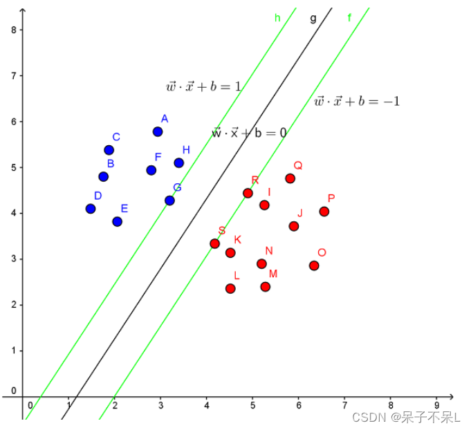
Support Vector Machine。支持向量机，其含义是通过支持向量运算的分类器。其中“机”的意思是机器，可以理解为分类器。 那么什么是支持向量呢？在求解的过程中，会发现只根据部分数据就可以确定分类器，这些数据称为支持向量。 见下图，在一个二维环境中，其中点R，S，G点和其它靠近中间黑线的点可以看作为支持向量，它们可以决定分类器，也就是黑线的具体参数。

解决的问题：

• 线性分类

在训练数据中，每个数据都有n个的属性和一个二类类别标志，我们可以认为这些数据在一个n维空间里。我们的目标是找到一个n-1维的超平面（hyperplane），这个超平面可以将数据分成两部分，每部分数据都属于同一个类别。 其实这样的超平面有很多，我们要找到一个最佳的。因此，增加一个约束条件：这个超平面到每边最近数据点的距离是最大的。也成为最大间隔超平面（maximum-margin hyperplane）。这个分类器也成为最大间隔分类器（maximum-margin classifier）。 支持向量机是一个二类分类器。

• 非线性分类

SVM的一个优势是支持非线性分类。它结合使用拉格朗日乘子法和KKT条件，以及核函数可以产生非线性分类器。

二、实战

1、画出决策边界

导包sklearn.svm

import numpy as np
import pandas as pd
import matplotlib.pyplot as plt
%matplotlib inline
 
# SVC: 分类
# SVR：回归
from sklearn.svm import SVC,SVR

随机生成数据，并且进行训练

• from sklearn.datasets import make_blobs

from sklearn.datasets import make_blobs
 
data,target = make_blobs(centers=2)
target
 
plt.scatter(data[:,0],data[:,1],c=target)

 创建SVC模型（使用线性核函数），并训练

# C=1.0, 惩罚系数，C越大越严格（有可能过拟合），C越小越不严格
# kernel='rbf', 核函数
        # linear：线性核函数，不常用
        # rbf：默认值，高斯核函数，基于半径的和函数，可以解决非线性问题
        # poly：多项式核函数
 
svc = SVC(C=1.0,kernel='linear')
 
svc.fit(data,target)

提取系数获取斜率

w1,w2 = svc.coef_[0]
w1,w2
# (1.0522835977410239, -0.8013229035839045)

线性方程的截距

b = svc.intercept_[0]
b
# 9.794733796740164

得到线性方程

# w1 * x1 + w2 * x2 + b = 0
 
# x2 作为y轴，x1作为x轴
# x2 = -(w1 * x1 + b) / w2

画图

plt.scatter(data[:,0],data[:,1],c=target)
 
x = np.linspace(data[:,0].min(),data[:,0].max(),20)
y =  -(w1 * x + b) / w2
 
plt.plot(x,y)

 

获取支持向量

svc.support_vectors_
'''
array([[-5.79772872,  5.85766345],
       [-4.59471853,  4.94156096]])
'''

画出支持向量所在直线

plt.scatter(data[:,0],data[:,1],c=target)
 
x = np.linspace(data[:,0].min(),data[:,0].max(),20)
y =  -(w1 * x + b) / w2
 
plt.plot(x,y)
 
# 画支持向量
vectors = svc.support_vectors_
plt.scatter(vectors[:,0],vectors[:,1],c='r',alpha=0.3,s=200)
 
 
# 活出支持向量所在的虚线
 
# vectors = array([[-4.64189396,  5.45729366],
#                 [-6.04692482,  7.04214351],
#                 [-3.63094168,  5.92881411],
#                 [-4.74569939,  7.93088232]])
 
b1 =  -(w1 * vectors[0,0] + w2 * vectors[0,1])
b2 =  -(w1 * vectors[1,0] + w2 * vectors[1,1])
 
y1 =  -(w1 * x + b1) / w2
y2 =  -(w1 * x + b2) / w2
 
plt.plot(x,y1,ls='--')
plt.plot(x,y2,ls='--')

 

2、使用多种核函数对iris数据集进行分类

导包

        from sklearn.datasets import load_iris

from sklearn.datasets import load_iris
 
 
data,target = load_iris(return_X_y=True)
 
data.shape
# (150, 4)

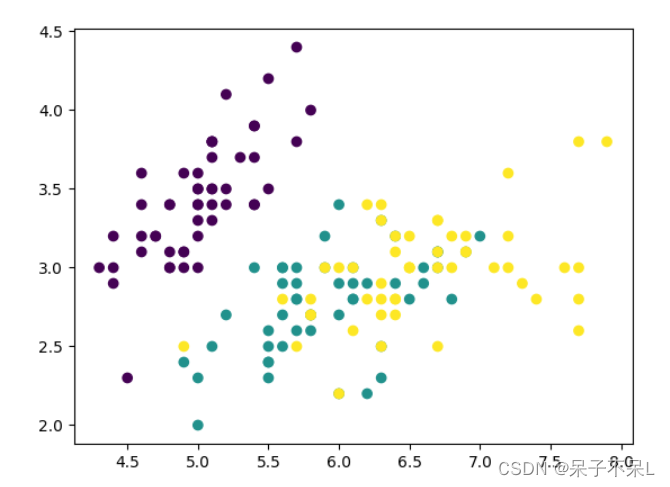
提取数据只提取两个特征，方便画图

data2 = data[:,:2].copy()
 
 
plt.scatter(data2[:,0],data2[:,1],c=target)

def get_XY(data2):
    x = np.linspace(data2[:,0].min(),data2[:,0].max(),1000)
    y = np.linspace(data2[:,1].min(),data2[:,1].max(),1000)
    X,Y = np.meshgrid(x,y)
    XY = np.c_[X.ravel(),Y.ravel()]
    return X,Y,XY
 
 
 
X,Y,XY = get_XY(data2)

创建支持向量机的模型：'linear', 'poly'(多项式), 'rbf'(Radial Basis Function:基于半径函数)

svc_dict = {
    'linear':SVC(kernel='linear'),
    'poly':SVC(kernel='poly'),
    'rbf':SVC(kernel='rbf')
}
 
 
for i,key in enumerate(svc_dict):
    # 训练
    svc = svc_dict[key]
    svc.fit(data2,target)
    
    # 预测
    y_pred = svc.predict(XY)
    
    # 画图
    axes = plt.subplot(1,3,i+1)
    axes.pcolormesh(X,Y,y_pred.reshape(1000,1000),shading='auto')
    axes.scatter(data2[:,0],data2[:,1],c = target,cmap='rainbow')
    
    axes.set_title(key,fontsize=20)

3、SVM分离坐标点

生成随机数据

data = np.random.randn(300,2)
data
 
plt.scatter(data[:,0],data[:,1])

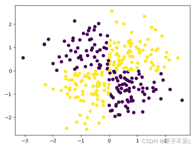
将1,3象限 和 2,4象限区分颜色

target = (data[:,0] * data[:,1] > 0) * 1
target
 
#  target = 1: 一三象限；target = 0：二四象限
'''
array([1, 1, 0, 0, 0, 0, 1, 1, 0, 1, 0, 1, 1, 0, 1, 1, 0, 1, 0, 1, 0, 1,
       1, 1, 1, 1, 0, 1, 1, 0, 0, 1, 0, 1, 1, 0, 0, 1, 1, 0, 0, 0, 0, 1,
       1, 1, 1, 0, 1, 1, 1, 1, 0, 0, 1, 1, 1, 1, 1, 1, 0, 0, 0, 1, 1, 0,
       1, 1, 1, 0, 0, 1, 1, 1, 1, 1, 0, 1, 0, 0, 1, 0, 1, 1, 1, 0, 0, 0,
       0, 0, 0, 0, 0, 1, 1, 0, 1, 0, 0, 0, 1, 0, 1, 0, 1, 1, 1, 0, 0, 0,
       0, 0, 1, 0, 0, 0, 1, 0, 0, 1, 1, 0, 1, 0, 1, 0, 0, 1, 0, 1, 1, 1,
       1, 0, 0, 1, 1, 0, 0, 0, 0, 1, 0, 0, 0, 0, 1, 0, 0, 1, 1, 0, 1, 0,
       0, 0, 1, 1, 0, 0, 0, 1, 1, 1, 1, 0, 0, 1, 1, 0, 0, 0, 0, 1, 1, 1,
       0, 0, 0, 0, 1, 1, 1, 1, 0, 1, 1, 0, 1, 1, 1, 0, 1, 1, 1, 1, 1, 0,
       1, 1, 0, 0, 1, 1, 0, 1, 0, 0, 1, 1, 1, 0, 1, 0, 1, 0, 1, 1, 0, 0,
       0, 1, 1, 1, 1, 1, 1, 0, 1, 0, 0, 1, 1, 0, 1, 1, 0, 0, 0, 1, 1, 0,
       0, 1, 1, 1, 1, 1, 0, 1, 1, 1, 1, 0, 1, 1, 1, 1, 1, 1, 0, 1, 0, 0,
       0, 0, 0, 0, 1, 0, 0, 0, 1, 1, 1, 0, 1, 1, 0, 1, 1, 1, 1, 1, 0, 1,
       1, 0, 0, 1, 0, 1, 1, 1, 0, 1, 0, 0, 1, 1])
'''
 
 
plt.scatter(data[:,0],data[:,1],c=target)

使用基于半径核函数

svc = SVC()
svc.fit(data,target)

创造一个范围的点以及meshgrid

def get_XY(data):
    x = np.linspace(data[:,0].min(),data[:,0].max(),1000)
    y = np.linspace(data[:,1].min(),data[:,1].max(),1000)
    X,Y = np.meshgrid(x,y)
    XY = np.c_[X.ravel(),Y.ravel()]
    return X,Y,XY
 
 
X,Y,XY = get_XY(data)

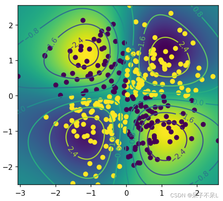
测试点到分离超平面的距离(decision_function)

distance = svc.decision_function(XY)
distance
'''
array([0.2733806 , 0.27487237, 0.27637551, ..., 0.33516833, 0.33292289,
       0.33069489])
'''

把距离当成一个二维的图片

画出图形

• 等高线
  • C = plt.contour(X, Y, distance.reshape(1000, 1000))

plt.figure(figsize=(5,5),dpi=150)
 
plt.imshow(distance.reshape(1000,1000),extent=[data[:,0].min(),data[:,0].max(),data[:,1].min(),data[:,1].max()])
 
# 等高线
C = plt.contour(X,Y,distance.reshape(1000,1000))
plt.clabel(C)   # 显示等高线
 
 
plt.scatter(data[:,0],data[:,1],c=target)

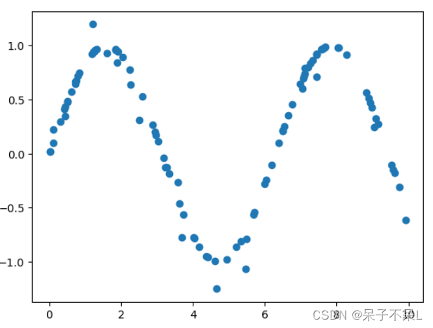
4、使用SVM多种核函数进行回归

自定义样本点rand，并且生成sin值

x = np.random.random(100) * 10
y = np.sin(x)
 
plt.scatter(x, y)

数据加噪

y[ : : 5] += np.random.randn(20) * 0.2
 
 
plt.scatter(x, y)

提供测试数据

x_test = np.linspace(0, 10, 100).reshape(-1, 1)

用不同的核函数预测

# linear
linear = SVR(kernel='linear')
linear.fit(x.reshape(-1, 1), y)
y_linear = linear.predict(x_test)
 
 
# poly
poly = SVR(kernel='poly')
poly.fit(x.reshape(-1, 1), y)
y_poly = poly.predict(x_test)
 
 
# rbf
rbf = SVR(kernel='rbf')
rbf.fit(x.reshape(-1, 1), y)
y_rbf = rbf.predict(x_test)
 
 
from sklearn.neighbors import KNeighborsRegressor
from sklearn.tree import DecisionTreeRegressor
 
 
# knn
knn = KNeighborsRegressor(n_neighbors=5)
knn.fit(x.reshape(-1, 1), y)
y_knn = knn.predict(x_test)
 
 
# tree
tree = DecisionTreeRegressor()
tree.fit(x.reshape(-1, 1), y)
y_ = tree.predict(x_test)

绘制图形，观察三种支持向量机内核不同

plt.scatter(x, y)
 
plt.plot(x_test, y_linear,  label='Linear')
plt.plot(x_test, y_poly,  label='poly')
plt.plot(x_test, y_rbf,  label='rbf')
plt.plot(x_test, y_knn,  label='knn')
plt.plot(x_test, y_,  label='tree')
 
plt.legend()