-
Oracle表格分类浅析1——普通堆表
说明:本文整理自书籍《收获,不止Oracle》
Oracle表的分类是多种多样的,除了普通表外,还有全局临时表、外部表、分区表、索引组织表等等具有其他特性的表。虽然普通表基本上可以实现所有的功能,但是这是说功能,而不是说性能。
如果我们善于在合适的场合选择合适的技术,这些“特殊”的表往往能在系统应用设计的性能方面,发挥出巨大的作用。
各种类型表都有优缺点,我们要善于取长补短,灵活利用,本篇文章,我们本着挑剔的态度来探讨普通表的缺点。
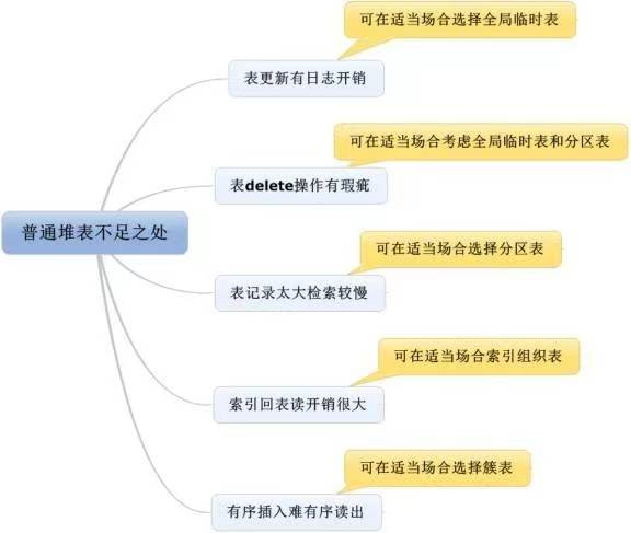
1. 表更新日志开销较大
如下语句可查询日志量:
select a.name,b.value from v$statname a,v$mystat b where a.statistic#=b.statistic# and a.name='redo size';- 1
- 2
- 3
- 4
为方便后续查询,我们创建如下视图:
--方便后续直接用select * from v$redo_size进行查询 create or replace view v$redo_size as select a.name,b.value from v$statname a,v$mystat b where a.statistic#=b.statistic# and a.name='redo size';- 1
- 2
- 3
- 4
- 5
- 6
- 7
- 8
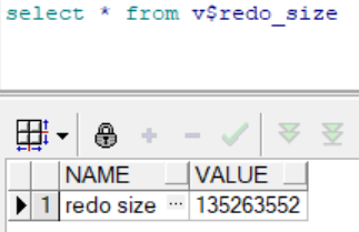
在进行实验前,我们可以先查询当前日志的大小,如下:
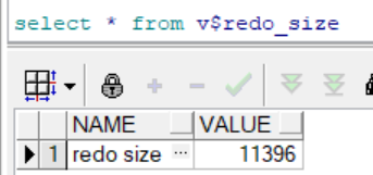
这个值的单位是字节数
现在开始实验,以观察DML操作产生的日志量。
1.1 建表
--建表 create table t as select*from dba_objects;- 1
- 2
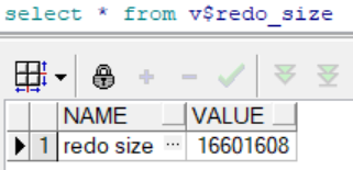
建表产生日志:
(16601608-11396)/1024/1024≈15.8M1.2 删除表数据
--删除表数据 delete from t;- 1
- 2
提交前

提交后

删除表数据产生日志:
(70055388-16601608)/1024/1024≈60M1.3 插入数据
--插入数据 insert into t select*from dba_objects;- 1
- 2
提交前
提交后

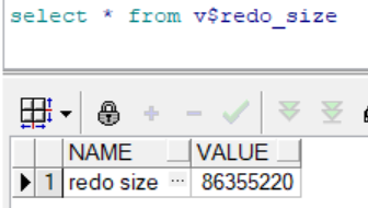
插入数据产生日志:
(86355360-70055388)/1024/1024≈15.5M1.4 更新数据
--更新数据 update t set object_id=rownum;- 1
- 2
提交前
提交后
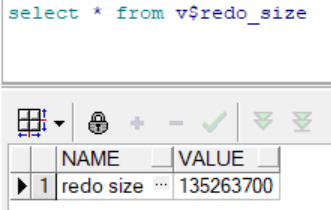
更新数据产生日志:
(135263700-86355360)/1024/1024≈46.6M这三个试验说明了对表的更新操作,无论是删除、插入还是修改,都会产生日志。
那么insert、update、delete三类语句,哪种记录redo log最多,哪种最少?
由上面的实验结果可以看出:delete产生的redo日志最多(60M),其次是update(46.6M),最少的是insert(15.5M)。2. delete无法释放空间
--查看执行计划 SQL> set autotrace on SQL> select count(*) from rui.t; COUNT(*) ---------- 141644 Execution Plan ---------------------------------------------------------- Plan hash value: 2966233522 ------------------------------------------------------------------- | Id | Operation | Name | Rows | Cost (%CPU)| Time | ------------------------------------------------------------------- | 0 | SELECT STATEMENT | | 1 | 559 (1)| 00:00:07 | | 1 | SORT AGGREGATE | | 1 | | | | 2 | TABLE ACCESS FULL| T | 140K| 559 (1)| 00:00:07 | ------------------------------------------------------------------- Note ----- - dynamic sampling used for this statement (level=2) Statistics ---------------------------------------------------------- 5 recursive calls 0 db block gets 2079 consistent gets 0 physical reads 0 redo size 528 bytes sent via SQL*Net to client 524 bytes received via SQL*Net from client 2 SQL*Net roundtrips to/from client 0 sorts (memory) 0 sorts (disk) 1 rows processed- 1
- 2
- 3
- 4
- 5
- 6
- 7
- 8
- 9
- 10
- 11
- 12
- 13
- 14
- 15
- 16
- 17
- 18
- 19
- 20
- 21
- 22
- 23
- 24
- 25
- 26
- 27
- 28
- 29
- 30
- 31
- 32
- 33
- 34
- 35
- 36
- 37
- 38
- 39
--删除数据后再次查看执行计划 SQL> set autotrace off SQL> delete from rui.t; 141644 rows deleted. SQL> commit; Commit complete. SQL> set autotrace on SQL> select count(*) from rui.t; COUNT(*) ---------- 0 Execution Plan ---------------------------------------------------------- Plan hash value: 2966233522 ------------------------------------------------------------------- | Id | Operation | Name | Rows | Cost (%CPU)| Time | ------------------------------------------------------------------- | 0 | SELECT STATEMENT | | 1 | 557 (1)| 00:00:07 | | 1 | SORT AGGREGATE | | 1 | | | | 2 | TABLE ACCESS FULL| T | 1 | 557 (1)| 00:00:07 | ------------------------------------------------------------------- Note ----- - dynamic sampling used for this statement (level=2) Statistics ---------------------------------------------------------- 4 recursive calls 0 db block gets 2079 consistent gets 0 physical reads 0 redo size 525 bytes sent via SQL*Net to client 524 bytes received via SQL*Net from client 2 SQL*Net roundtrips to/from client 0 sorts (memory) 0 sorts (disk) 1 rows processed- 1
- 2
- 3
- 4
- 5
- 6
- 7
- 8
- 9
- 10
- 11
- 12
- 13
- 14
- 15
- 16
- 17
- 18
- 19
- 20
- 21
- 22
- 23
- 24
- 25
- 26
- 27
- 28
- 29
- 30
- 31
- 32
- 33
- 34
- 35
- 36
- 37
- 38
- 39
- 40
- 41
- 42
- 43
- 44
- 45
- 46
- 47
- 48
- 49
记录数从141644减少到0条记录了,为什么逻辑读还是2079呢?
我们先继续下面的实验:
SQL> truncate table rui.t; Table truncated. SQL> select count(*) from rui.t; COUNT(*) ---------- 0 Execution Plan ---------------------------------------------------------- Plan hash value: 2966233522 ------------------------------------------------------------------- | Id | Operation | Name | Rows | Cost (%CPU)| Time | ------------------------------------------------------------------- | 0 | SELECT STATEMENT | | 1 | 2 (0)| 00:00:01 | | 1 | SORT AGGREGATE | | 1 | | | | 2 | TABLE ACCESS FULL| T | 1 | 2 (0)| 00:00:01 | ------------------------------------------------------------------- Note ----- - dynamic sampling used for this statement (level=2) Statistics ---------------------------------------------------------- 6 recursive calls 1 db block gets 13 consistent gets 0 physical reads 96 redo size 525 bytes sent via SQL*Net to client 524 bytes received via SQL*Net from client 2 SQL*Net roundtrips to/from client 0 sorts (memory) 0 sorts (disk) 1 rows processed- 1
- 2
- 3
- 4
- 5
- 6
- 7
- 8
- 9
- 10
- 11
- 12
- 13
- 14
- 15
- 16
- 17
- 18
- 19
- 20
- 21
- 22
- 23
- 24
- 25
- 26
- 27
- 28
- 29
- 30
- 31
- 32
- 33
- 34
- 35
- 36
- 37
- 38
- 39
- 40
- 41
这里很显然看出:
- delete 删除并不能释放空间,虽然delete将很多块的记录删除了,但是空块依然保留,Oracle 在查询时依然会去查询这些空块。
- truncate 是一种释放高水平位的动作,这些空块被回收,空间也就释放了。
举个简单的例子,好比我来到XX大楼统计里面的人数,我从1楼找到20楼,每层的房间都打开去检查了一下,发现实际情况是一个人都没有。我很后悔自己累得半死却得出没人的结论,但问题是,你不打开房间,怎么知道没人呢,这就类似delete后空块的情况。而与truncate有些类似的生动例子就是,我想统计 XX 大楼里的人数,结果发现,XX 大楼被铲平了,啥房间都没有了,于是我飞快地得出结论,XX大楼里没有人。
不过truncate显然不能替代delete,因为truncate是一种DDL操作而非DML操作,truncate后面是不能带条件的,truncate table t where…是不允许的。
但是如果表中这些where条件能形成有效的分区,Oracle是支持在分区表中做truncate分区的,命令大致为 alter table t truncate partition ‘分区名’,如果where条件就是分区条件,那等同于换角度实现了truncate table t where…的功能。当大量delete 删除再大量insert插入时,Oracle会去这些delete的空块中首先完成插入(直接路径插入除外),所以频繁delete又频繁insert的应用,是不会出现空块过多的情况的。
3. 表记录太大检索较慢
一张表其实就是一个SEGMENT,一般情况下我们都需要遍历该SEGMENT的所有BLOCK来完成对该表进行更新查询等操作,在这种情况下,表越大,更新查询操作就越慢!
有没有什么好方法能提升检索的速度呢?主要思路就是缩短访问路径来完成同样的更新查询操作,简单地说就是完成同样的需求访问BLOCK的个数越少越好。Oracle为了尽可能减少访问路径提供了两种主要技术,一种是索引技术,另一种则是分区技术。
我们先来说说索引技术:
当我们建成了一个索引,在SQL查询时我们首先会访问索引段,然后通过索引段和表段的映射关系,迅速从表中获取行列的信息并返回结果。再来说说分区技术:
分区技术就是把普通表T表改造为分区表,比如以select * from t where created>= xxx and created <=xxx 这个简单的SQL语句为例进行分析。
如果以created这个时间列为分区字段,比如从2010年1月到2012年12月按月建36个分区。早先的T表就一个T段,现在情况变化了,从1个大段分解成了36个小段,分别存储了2010年1月到2012年12月的信息,此时假如created>= xxx and created <=xxx 这个时间跨度正好是落在2012年11月,那Oracle的检索就只要完成一个小段的遍历即可,假设这36个小段比较均匀,我们就可以大致理解为访问量只有原来的三十六分之一,大幅度减少了访问路径,从而高效地提升了性能。4. 索引回表读开销很大
SQL> drop table rui.t purge; Table dropped. SQL> create table rui.t as select * from dba_objects where rownum <= 200; Table created. SQL> create index idx_obj_id on rui.t(object_id); Index created. SQL> set linesize 1000 SQL> set autotrace traceonly SQL> select * from rui.t where object_id<=10; 9 rows selected. Execution Plan ---------------------------------------------------------- Plan hash value: 134201588 ------------------------------------------------------------------------------------------ | Id | Operation | Name | Rows | Bytes | Cost (%CPU)| Time | ------------------------------------------------------------------------------------------ | 0 | SELECT STATEMENT | | 9 | 1863 | 2 (0)| 00:00:01 | | 1 | TABLE ACCESS BY INDEX ROWID| T | 9 | 1863 | 2 (0)| 00:00:01 | |* 2 | INDEX RANGE SCAN | IDX_OBJ_ID | 9 | | 1 (0)| 00:00:01 | ------------------------------------------------------------------------------------------ Predicate Information (identified by operation id): --------------------------------------------------- 2 - access("OBJECT_ID"<=10) Note ----- - dynamic sampling used for this statement (level=2) Statistics ---------------------------------------------------------- 23 recursive calls 0 db block gets 40 consistent gets 0 physical reads 0 redo size 2318 bytes sent via SQL*Net to client 524 bytes received via SQL*Net from client 2 SQL*Net roundtrips to/from client 0 sorts (memory) 0 sorts (disk) 9 rows processed- 1
- 2
- 3
- 4
- 5
- 6
- 7
- 8
- 9
- 10
- 11
- 12
- 13
- 14
- 15
- 16
- 17
- 18
- 19
- 20
- 21
- 22
- 23
- 24
- 25
- 26
- 27
- 28
- 29
- 30
- 31
- 32
- 33
- 34
- 35
- 36
- 37
- 38
- 39
- 40
- 41
- 42
- 43
- 44
- 45
- 46
- 47
- 48
- 49
- 50
- 51
- 52
- 53
- 54
- 55
注意执行计划中有“TABLE ACCESS BY INDEX ROWID”关键字。
一般来说,根据索引来检索记录,会有一个先从索引中找到记录,再根据索引列上的ROWID定位到表中从而返回索引列以外的其他列的动作,这就是TABLE ACCESS BY INDEX ROWID 。
SQL> select object_id from rui.t where object_id<=10; 9 rows selected. Execution Plan ---------------------------------------------------------- Plan hash value: 188501954 ------------------------------------------------------------------------------- | Id | Operation | Name | Rows | Bytes | Cost (%CPU)| Time | ------------------------------------------------------------------------------- | 0 | SELECT STATEMENT | | 9 | 117 | 1 (0)| 00:00:01 | |* 1 | INDEX RANGE SCAN| IDX_OBJ_ID | 9 | 117 | 1 (0)| 00:00:01 | ------------------------------------------------------------------------------- Predicate Information (identified by operation id): --------------------------------------------------- 1 - access("OBJECT_ID"<=10) Note ----- - dynamic sampling used for this statement (level=2) Statistics ---------------------------------------------------------- 7 recursive calls 0 db block gets 10 consistent gets 0 physical reads 0 redo size 637 bytes sent via SQL*Net to client 524 bytes received via SQL*Net from client 2 SQL*Net roundtrips to/from client 0 sorts (memory) 0 sorts (disk) 9 rows processed- 1
- 2
- 3
- 4
- 5
- 6
- 7
- 8
- 9
- 10
- 11
- 12
- 13
- 14
- 15
- 16
- 17
- 18
- 19
- 20
- 21
- 22
- 23
- 24
- 25
- 26
- 27
- 28
- 29
- 30
- 31
- 32
- 33
- 34
- 35
- 36
- 37
- 38
- 39
执行计划中没有“没有TABLE ACCESS BY INDEX ROWID”关键字了!
因为语句从 select * from t where object_id<=10 改写为 select object_id from t where object_id<=10 了,不用从索引中回到表中获取索引列以外的其他列了。
可以发现性能有所提升。
避免回表从而使性能提升这是一个很简单的道理,少做事性能当然提升了。只是select* from t 和select object_id from t毕竟不等价,有没有什么方法可以实现写法依然是select * from t,但是还是可以不回表呢?
普通表是做不到的,能实现这种功能的只有索引组织表。
5. 有序插入却难有序读出
在对普通表的操作中,我们无法保证在有序插入的前提下就能有序读出。最简单的一个理由就是,如果你把行记录插入块中,然后删除了该行,接下来插入的行会去填补块中的空余部分,这就无法保证有序了。实验如下:
SQL> drop table rui.t purge; Table dropped. SQL> create table rui.t (a int,b varchar2(4000)default rpad('*',4000,'*'),c varchar2(3000)default rpad('*',3000,'*')); Table created. SQL> insert into rui.t (a) values (1); 1 row created. SQL> insert into rui.t (a) values (2); 1 row created. SQL> insert into rui.t (a) values (3); 1 row created. SQL> select A from rui.t; A ---------- 1 2 3 SQL> delete from rui.t where a=2; 1 row deleted. SQL> insert into rui.t (a) values (4); 1 row created. SQL> select A from rui.t; A ---------- 1 4 3- 1
- 2
- 3
- 4
- 5
- 6
- 7
- 8
- 9
- 10
- 11
- 12
- 13
- 14
- 15
- 16
- 17
- 18
- 19
- 20
- 21
- 22
- 23
- 24
- 25
- 26
- 27
- 28
- 29
- 30
- 31
- 32
- 33
- 34
- 35
- 36
- 37
- 38
- 39
- 40
- 41
- 42
因为BLOCK大小默认是8KB,所以这里特意用rpad(‘‘,4000,’’), rpad(‘‘,3000,’’)来填充B、C字段,这样可以保证一个块只插入一条数据,方便做试验分析跟踪。
我们在查询数据时,如果想有序地展现,就必须使用order by ,否则根本不能保证顺序展现,而order by 操作是开销很大的操作,实验如下:
--order by 操作是开销很大的操作 SQL> set linesize 1000 SQL> set autotrace traceonly SQL> select A from rui.t; Execution Plan ---------------------------------------------------------- Plan hash value: 1601196873 -------------------------------------------------------------------------- | Id | Operation | Name | Rows | Bytes | Cost (%CPU)| Time | -------------------------------------------------------------------------- | 0 | SELECT STATEMENT | | 3 | 39 | 3 (0)| 00:00:01 | | 1 | TABLE ACCESS FULL| T | 3 | 39 | 3 (0)| 00:00:01 | -------------------------------------------------------------------------- Note ----- - dynamic sampling used for this statement (level=2) Statistics ---------------------------------------------------------- 0 recursive calls 0 db block gets 7 consistent gets 0 physical reads 0 redo size 581 bytes sent via SQL*Net to client 524 bytes received via SQL*Net from client 2 SQL*Net roundtrips to/from client 0 sorts (memory) 0 sorts (disk) 3 rows processed SQL> select A from rui.t order by A; Execution Plan ---------------------------------------------------------- Plan hash value: 961378228 --------------------------------------------------------------------------- | Id | Operation | Name | Rows | Bytes | Cost (%CPU)| Time | --------------------------------------------------------------------------- | 0 | SELECT STATEMENT | | 3 | 39 | 4 (25)| 00:00:01 | | 1 | SORT ORDER BY | | 3 | 39 | 4 (25)| 00:00:01 | | 2 | TABLE ACCESS FULL| T | 3 | 39 | 3 (0)| 00:00:01 | --------------------------------------------------------------------------- Note ----- - dynamic sampling used for this statement (level=2) Statistics ---------------------------------------------------------- 4 recursive calls 0 db block gets 15 consistent gets 0 physical reads 0 redo size 581 bytes sent via SQL*Net to client 524 bytes received via SQL*Net from client 2 SQL*Net roundtrips to/from client 1 sorts (memory) 0 sorts (disk) 3 rows processed- 1
- 2
- 3
- 4
- 5
- 6
- 7
- 8
- 9
- 10
- 11
- 12
- 13
- 14
- 15
- 16
- 17
- 18
- 19
- 20
- 21
- 22
- 23
- 24
- 25
- 26
- 27
- 28
- 29
- 30
- 31
- 32
- 33
- 34
- 35
- 36
- 37
- 38
- 39
- 40
- 41
- 42
- 43
- 44
- 45
- 46
- 47
- 48
- 49
- 50
- 51
- 52
- 53
- 54
- 55
- 56
- 57
- 58
- 59
- 60
- 61
- 62
- 63
- 64
- 65
- 66
- 67
- 68
- 69
可以观察到,有排序的操作的统计信息模块有一个1 sorts (memory),表示发生了排序,执行计划中也有SORT ORDER BY的关键字,不过最重要的是,没排序的操作代价为3,有排序的操作代价为4,性能上是有差异的,在大数量时将会非常明显。
关于order by 避免排序的方法有两种思路。
第一种思路是在order by 的排序列建索引。
第二种方法就是,将普通表改造为有序散列聚簇表,这样可以保证顺序插入,order by 展现时无须再有排序动作。 -
相关阅读:
Docker快速入门到项目部署,docker自定义镜像
react的高阶组件怎么用?
Nacos客户端启动出现9848端口错误分析(非版本升级问题)
年度盘点,四年的精华合集「GitHub 热点速览」
【MAPBOX基础功能】12、mapbox点击点位图层高亮指定的点位
西工大&ANU&CSIRO&IIAI提出基于排序的伪装目标检测网络RankNet,并提供了最大的COD数据集!...
Git常用命令
基于x86架构的CentOS7虚拟机通过qemu安装ARM架构CentOS7虚拟机
C#webform Static DataTable 多人同时操作网页数据重复问题
高程复习 欧几里得算法和扩展欧几里得算法考试前冲刺简约版
- 原文地址:https://blog.csdn.net/Ruishine/article/details/127432696
